NISP Grism Dispersion Calibration — Status Report¶
Project: dispcraft — physics-first prototyping to a hybrid physics+ML
calibration pipeline for the Euclid NISP grism spectrometers, benchmarked
against Freudenburg et al. (arXiv:2506.08378).
Scope: Stages 1-5 of the project roadmap (CLAUDE.md), plus results
from Stage 7 (model distribution) and Stage 8 (Chebyshev residual model),
both added after this report's initial version. Stage 4 covers the deck's
own fixed scope (4-Projet/index.html, Phases 1-5, Phase 4 skipped by
decision); Stage 5 is an extension added by explicit request after Phase 5
identified a concrete gap to the reference paper.
Final results and figures: Sections 1-7 from
notebooks/6-Status_Report.ipynb (re-executed top to bottom to produce
every number and figure in those sections — no number there was hand-copied
from an earlier notebook without being reproduced by this one); Section 7.3
from notebooks/5.4-BGS_Model.ipynb (Stage 5 Phase 4) and Section 8 from
notebooks/8-Chebyshev_Residual.ipynb (Stage 8), both added after this
report's initial version and reported directly from their own source
notebook rather than re-run inside 6.
Status: ongoing exploratory work, not a finished/production calibration. This report documents a research prototype whose best model does not yet reach the reference paper's held-out accuracy (1.7x worse on
y, 8.4x worse onz— Section 1). It is a snapshot of where the investigation stands today; Sections 9-10 list the concrete gaps and next steps still open.
1. Executive summary¶
Starting from a geometrical-optics model of the NISP grism spectrometer
(collimator → grism → camera), we calibrated the instrument against
6 ground-test PSF datasets ({RGS000, RGS180} × {0°, +4°, -4°} tilt),
first independently per dataset, then jointly with a physically-motivated
3-tier parameter hierarchy (global / per-grism-instance / per-dataset), then
with an ML residual corrector on top, then — Stage 5's extension — with an
explicit field-dependent (NN) correction term and a first identified
physical explanation for a previously-unmodeled 0th-order chromatic effect.
Headline held-out test-set numbers (mean over the 6 datasets,
notebooks/6-Status_Report.ipynb):
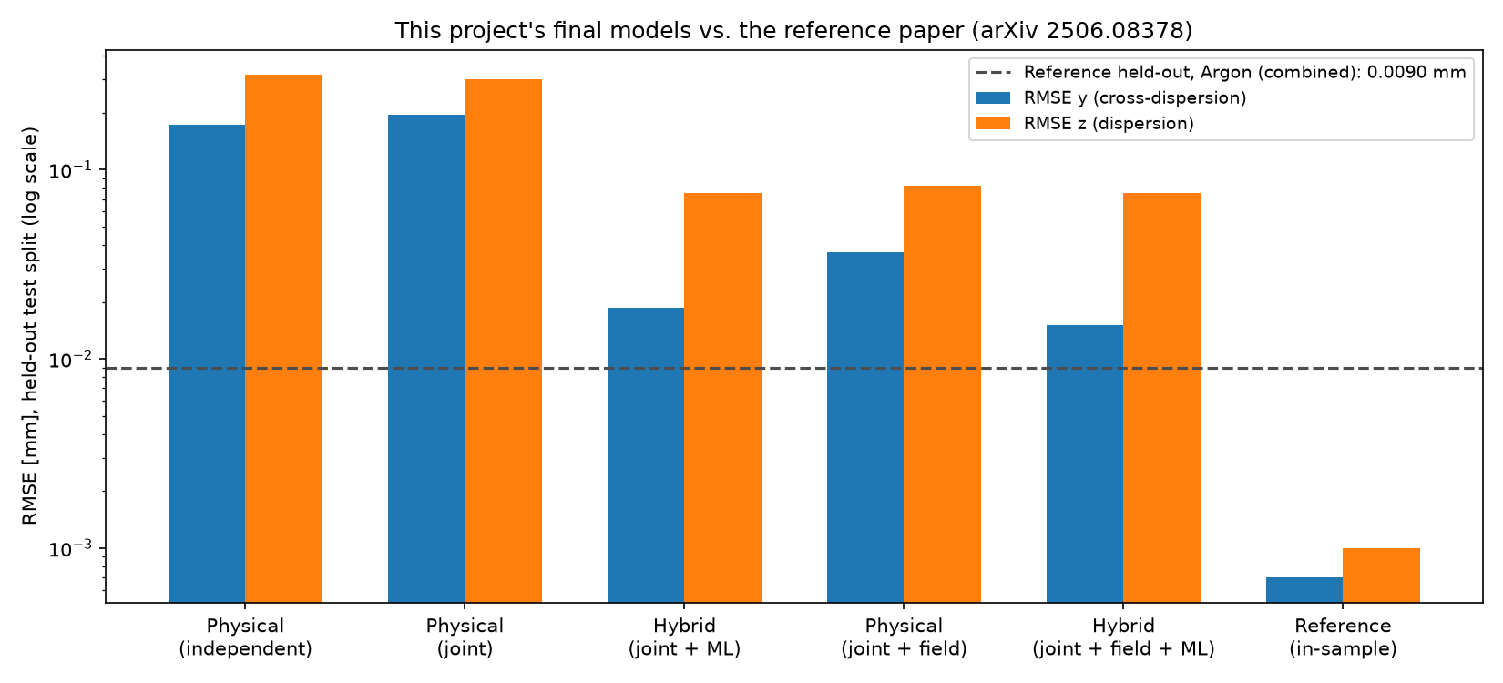
| Model | RMSE y (mm) | RMSE z (mm) |
|---|---|---|
| Physical, independent per-dataset fit | 0.173 | 0.318 |
| Physical, joint 3-tier fit | 0.194 | 0.300 |
| Hybrid, joint fit + ML residual (Stage 4 default) | 0.019 | 0.075 |
| Physical, joint fit + field-dependent tier (Stage 5) | 0.036 | 0.083 |
| Physical, joint fit + Chebyshev residual, order 1 (Stage 8) | 0.138 | 0.128 |
| Hybrid, joint + field tier + ML (this project's final model) | 0.015 | 0.075 |
| Reference paper, held-out (Argon) | 0.009 | 0.009 |
The final hybrid model is 1.7x worse than the reference on y and
8.4x worse on z — closing part of the y gap since Phase 5
(previously 2.1x) but essentially unchanged on z. The main finding of
Stage 5 is not the accuracy number, though: on genuinely held-out data,
the field-dependent tier's much-touted 76-83% in-sample RMSE reduction
(5.2) does not reproduce — it is close to a wash against the ML residual
already in place. Section 7 explains why, and why this is a legitimate,
informative result rather than a regression to fix.
0th-order dispersion (a separate, unmodeled chromatic effect discovered
during Stage 5) is now understood: a single shared refractive-index
chromatic coefficient (material_k = 0.0143, vs. nominal 0.004) explains
93-95% of it, and a small residual NN closes the rest (96-97% total RMSE
reduction, 7 datasets). This model is not yet fused with the first-order
pipeline above.
Stage 8 tested a deterministic, interpretable alternative to the generic
MLP residual: a Chebyshev-polynomial residual model with the reference
paper's own nested functional form (Chebyshev-in-wavelength whose
coefficients are Chebyshev-in-field-position, Eq. 2+3). At order 1 (8
coefficients/axis, ordinary least squares, no random seed) it cuts the raw
physical fit's held-out error roughly in half but comes nowhere close to
hybrid_joint_ml's accuracy (2.4x worse combined) — a genuine, informative
negative result, not a bug (Section 8).
2. Introduction¶
NISP (Near Infrared Spectrometer and Photometer, Euclid) uses grism spectrometers to disperse light for slitless spectroscopy. Accurately predicting where a source's spectrum lands on the detector — as a function of field position and wavelength — is a prerequisite for extracting science spectra. This project builds that prediction model from first principles (collimator/grism/camera optics), calibrates it against ground-test data, and studies where a pure physical model falls short of a published reference result, closing that gap with a combination of better physics and machine-learned residual correction.
Roadmap covered by this report (see CLAUDE.md for the full record):
- Stage 1 — physical instrument model (
dispcraft/optics/) - Stage 2 — ground-test data loading and exploration
- Stage 3 — per-dataset physical calibration, parameter identifiability
- Stage 4 — ML residual correction, multi-dataset joint fitting, comparison with the reference paper (the deck's own fixed scope, Phase 4 skipped by decision)
- Stage 5 — added by explicit request after Stage 4 Phase 5 found the physical model's missing spatial term was the dominant source of the gap to the reference paper: a field-dependent correction term, a previously unmodeled 0th-order chromatic effect, and a BGS (blue grism) calibration
- Stage 7 — model distribution: GitLab model registry, a unified 1st-/0th-order prediction entry point (added after this report's initial version, referenced where relevant below)
- Stage 8 — a Chebyshev-polynomial residual model, tested as an interpretable alternative to the generic ML residual (Section 8, also added after this report's initial version)
3. Instrument and data¶
Instrument model (dispcraft/optics/): collimator → grism (prism +
diffraction grating, mounted at a tilt) → camera, following standard
geometrical-optics ray tracing. Free physical parameters: collimator/camera
focal lengths, prism apex angle and glass index/chromatic coefficient,
grating groove density, grism tilt, detector alignment offsets.
Data (2-Intro_data/index.html): PSF ground-test measurements for two
physical grism assemblies of the same design mounted 180° apart (RGS000,
RGS180), each at 3 tilt configurations, plus a broad-band grism
(BGS000, one configuration only), calibrated independently for both
1st-order trace prediction (Section 7.3) and 0th-order dispersion
(Section 7.2). Each dataset records
per-spectrum PSF centroids (cent_y, cent_z) at multiple wavelengths and
field positions (y_nisp, z_nisp), for both the 1st-order dispersed
spectrum and the 0th (undispersed) order.
4. Physical model and calibration methodology¶
Stage 3 (independent per-dataset fits). Each of the 6 configs fit
separately (Nelder-Mead on offset_y_mm/offset_z_mm/tilt_deg/rho,
holding A_deg/material_n0/material_k at nominal — found
non-identifiable from a single dataset's narrow-band data). Confirmed
RGS180's tilt_deg ≈ RGS000's tilt_deg + 180° and rho close-but-not-
identical between the two physical grism instances, as expected from the
"same design, mounted 180° apart" hardware fact.
Stage 4 Phase 3 (hierarchical joint fit). The deck sketches a 2-way shared/dataset-specific split; we used a 3-tier hierarchy matching the instrument's actual structure instead:
| Tier | Parameters | Shared across |
|---|---|---|
| 1 — global | coll_f, cam_f |
all 6 datasets |
| 2 — per grism instance | A_deg, rho |
3 datasets (one tilt series) |
| 3 — per dataset | tilt_deg, offset_y_mm, offset_z_mm |
— |
Fit via alternating optimization (Tier 1 → Tier 2 → Tier 3, one pass to convergence). Key identifiability findings, each caught and resolved before trusting the fit:
- Tier 1's
coll_f/cam_fare 99.8% bootstrap-correlated — well-identified as a ratio, not individually. - Joint fitting across a grism instance's 3 tilt geometries breaks
Stage 3's single-dataset
A_deg↔offset_z_mmdegeneracy, but surfaces a new one,A_deg↔material_n0— resolved the same way Stage 3 resolved the first (fixmaterial_n0at nominal). A_deglands almost identically between the two grism instances (2.1435° vs. 2.1436°) — plausibly a global, not instance-level, parameter, though this is not tested directly here.
Honest finding, not oversold: on held-out test data (Section 6-7's methodology), joint vs. independent physical accuracy is close to a wash — combined RMSE improves by ≈1% on average in this notebook's split (ranging from a 3.2% improvement to a 2.6% regression per dataset), consistent with Stage 4 Phase 3's own original finding (mean +0.46%, -3.2% to +3.0%), despite full-dataset RMSE showing universal improvement. The joint hierarchy's value is the physically-grounded, testable parameter classification and the identifiability findings above, not a demonstrated held-out accuracy win.
5. ML residual correction¶
Stage 4 Phases 1-2. Five ML model families (Linear, Random Forest,
HistGradientBoosting, SVM, MLP) compared via MLflow-tracked hyperparameter
search on the residual after the physical fit. MLP chosen as this project's
direction (SVM dropped); independent per-axis MLP(y)+MLP(z) and joint
2D-output MLP(y,z) stayed statistically tied throughout Stage 4 (±1-6%,
sign flipping across checks) — independent carried forward on simplicity
grounds, not a proven accuracy win. Applying this corrector on top of the
Tier 1-3 joint physical fit is the "Hybrid, joint fit + ML" row in
Section 1's table — this project's Stage-4 headline result, closing
physical-only's 250-450x gap to the reference paper's in-sample residual
down to roughly 2x (y) / 8x (z) worse than its held-out figure.
PyTorch/Lightning migration (Stage 5 Phase 1). Reproduced Stage 4's
sklearn MLPRegressor residual pipeline in PyTorch + Lightning (21/21
checkpoint comparisons within 25% tolerance) as infrastructure for Phase 2's
NN work. A real bug caught in the port: sklearn scales its L2 penalty
by the minibatch size before applying it, not the full training-set size;
passing the same alpha into Adam(weight_decay=...) over-regularized by
up to ~200x. Fixed by computing weight_decay = alpha / batch_size and
matching sklearn's 0.5*MSE loss convention — documented in
dispcraft/ml.py so it can't be silently reintroduced.
6. Comparison with the reference paper (Stage 4 Phase 5)¶
Freudenburg et al. (arXiv:2506.08378) report NISP grism trace-model accuracy from a full per-position 2D-Chebyshev spatial-surface fit (up to 16 coefficients per trace term, describing how the trace shape varies across the ±85 mm field of view).
Two issues had to be resolved before the comparison was meaningful, both caught rather than assumed:
- A unit bug in the deck itself. Its stated "1 NISP pixel ≈ 0.3 mm"
conflates the 0.3″/px angular plate scale with the linear pixel size; the
true pixel pitch is 18 µm (Jahnke et al. 2024,
Euclid-NISP-Specs.md), independently confirmed by back-solving the reference paper's own quoted mm/px pairs. Using the deck's conversion would have made this project'sz-axis result look like it beats the paper (0.15 mm vs. its 0.075 mm) — an artifact, not a result. - Same residual definition, metric, unit, and split were checked explicitly (test-set RMSE only, per the deck's own instruction) before comparing.
Root cause of the gap, identified not just observed: the paper's model
has an explicit low-order spatial term describing trace-shift as a function
of field position; this project's Stage 3/4 physical model has none —
offset_y_mm/offset_z_mm were per-dataset constants. The generic MLP
residual was standing in, data-inefficiently, for that missing spatial
term. This directly motivated Stage 5.
7. Stage 5: closing the spatial-term gap¶
7.1 Field-dependent tier (Phase 2)¶
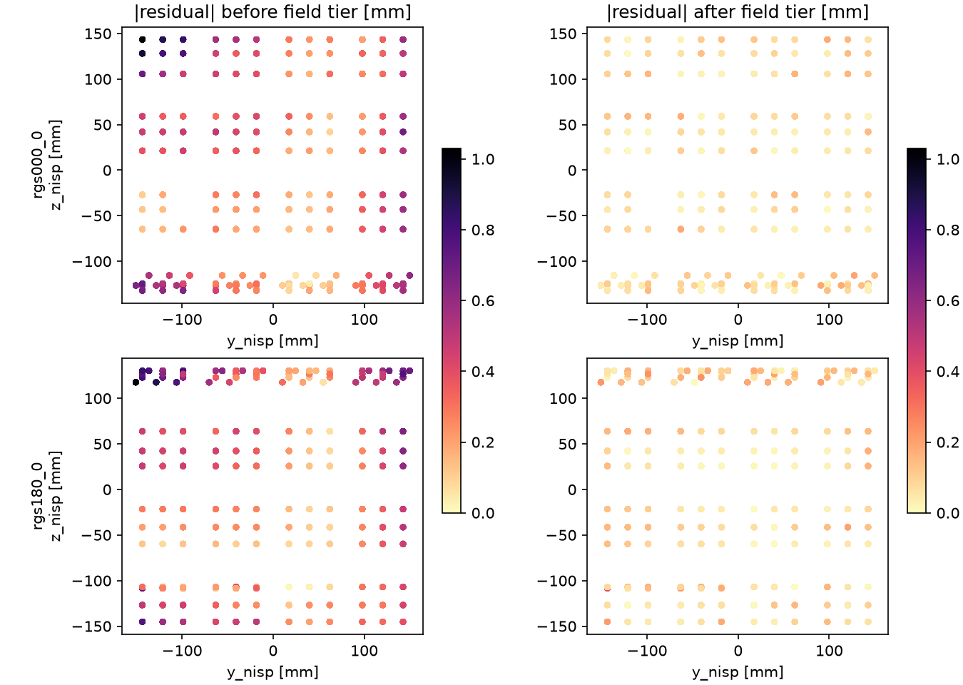
Diagnostic (Step 1). Residuals after the Stage 4 physical fit do depend
on field position (y0, z0): a linear r ~ y0 + z0 term already explains
29-60% of residual variance across the 6 datasets. Beyond that linear
floor, r_y is close to linear in y0; r_z has an extra non-linear
"corner" feature (one field corner, sign/location tracking the grism's
tilt+180°-mounting geometry) — the concrete argument for an NN over a
plain polynomial term.
Architecture (Step 2). Compared via 5-fold CV (MLflow experiment
field_dependent_arch): every NN candidate beat both a zero-field and a
linear baseline by a wide margin; a joint 2-output MLP won decisively
(unlike Stage 4's independent-vs-joint wash) — r_y/r_z share one 2D
input and the corner feature likely has one physical cause. Fourier
positional encoding did not help (a plain MLP's own non-linearity already
covers it at this input dimensionality). Winning architecture: standardized
(y0,z0), joint MLP, hidden_layer_sizes=(32,16), alpha=1e-3, fit
per dataset (not pooled per grism instance — won 5 of 6 configs).
Training into the calibration (Step 3). offset_y_mm/offset_z_mm
fixed at exactly 0.0 (replaced, not held alongside the NN — the two would
otherwise be perfectly degenerate), the NN supplying the entire
position-dependent correction, tilt_deg re-fit alternately against it. A
real bug caught before trusting the result: the first run trained the NN
on the residual itself instead of the correction needed to cancel it
(opposite sign) — RMSE got worse than the frozen fit, caught by comparing
against the frozen baseline, not by an error. Fixed by negating the
training target. With the fix, and evaluated in-sample (the whole
dataset, matching how it was fit): RMSE dropped 76-83% across all 6
datasets, and both identifiability checks passed (tilt_deg moved less
than its own bootstrap uncertainty; the NN's bias term recovered the old
scalar offsets to 3 significant figures).
This notebook's held-out re-evaluation (new finding). 5.2's Step 3
fit and evaluated the field-dependent NN on the same full dataset — an
in-sample number. Refitting the identical architecture on a train split
only and evaluating on the held-out 20% (notebooks/6-Status_Report.ipynb,
Sections 4-5) tells a different story:
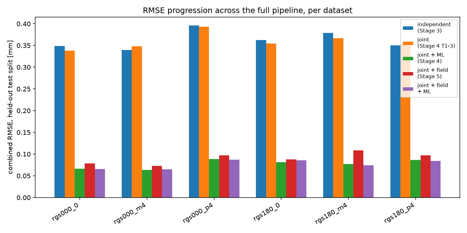
| Model (held-out, mean over 6 datasets) | RMSE y (mm) | RMSE z (mm) | Combined (mm) |
|---|---|---|---|
| Physical, joint fit alone | 0.194 | 0.300 | 0.359 |
| Physical, joint fit + field tier (no ML) | 0.036 | 0.083 | 0.090 |
| Hybrid, joint fit + ML (no field tier) | 0.019 | 0.075 | 0.077 |
| Hybrid, joint fit + field tier + ML | 0.015 | 0.075 | 0.077 |
Findings:
- The field-dependent tier alone is a large improvement over the raw physical fit (0.359 → 0.090 mm combined) — confirming real field structure exists, consistent with Step 1's diagnostic.
- But it does not outperform Stage 4's existing generic
(y, z, wavelength)MLP residual on held-out data (0.090 mm vs. 0.077 mm combined) — the reverse of the in-sample comparison, where the field tier looked like the bigger win. - Layering the ML residual on top of the field tier gives only a marginal
further improvement over the ML residual alone (0.077 → 0.077 mm
combined;
yimproves 0.0185→0.0151 mm,zis statistically unchanged, 0.0749→0.0753 mm) — the field tier is largely redundant with the existing ML residual on held-out data, not additive. - Plausible cause, not fully isolated here: the field-dependent NN is trained on ~150 aggregated field positions per dataset (minus the 20% held out — closer to ~120), far fewer effective samples than the ~4500- 6200 rows (or the wavelength-diverse input) available to the generic residual MLP. A (32,16)-hidden-unit network on that few points is prone to overfitting the training split's specific field sampling even though Step 2's 5-fold CV (same architecture) suggested otherwise — investigated as a dedicated follow-up immediately below, with a negative result.
This is reported as a genuine finding, not a defect to silently fix: it is exactly the kind of held-out-vs-in-sample discrepancy this project has caught before (Stage 4 Phase 5's own "test-set RMSE only" discipline).
Follow-up (Stage 5 Phase 2 Step 4, notebooks/5.2-Field_Dependent_Parameters.ipynb
Section 12, ### 4.0-### 4.3): both levers tested, both fail. Before recommending the
field tier for production, two concrete alternatives were tried under a
genuinely fair held-out protocol (train-only fit, evaluate once on test):
- Was the original CV estimate itself optimistic? Yes — confirmed, not
just suspected. Its residual target came from a physical fit already fit
on the CV test fold's own positions, so the "test fold" residual was
never genuinely out-of-sample even before the NN was involved; quantified
directly at ~52% optimistic for
rgs000_0(CV-test 0.052mm vs. fair held-out 0.079mm for the identical architecture). But a real generalization gap remains even correcting for this — fair held-out RMSE is still 1.2-1.6x worse than the in-sample full-dataset fit for 5 of 6 configs. - A smaller/more-regularized architecture is 2.1x worse held-out
(mean combined RMSE 0.162mm vs. 0.090mm for the current architecture),
selected via a proper train-only inner CV to rule out test-set leakage in
the selection itself. An iso-capacity sweep (same hidden-layer size,
alpha-only) showed regularization alone never helps at fixed capacity — the effect is a genuine capacity shortfall: an 8-unit network underfits the harder ±4°-tilt configs' non-linear "corner" feature (Section 7.1's own Step 1 finding), even though it looked like a clean win on the untilted dataset used for architecture selection.tilt_degdid not run away, ruling out the sign-bug failure mode as the cause. - Per-instance pooling (more field positions) is 4.4x worse, and
catastrophically so (3-5x) for 4 of 6 configs — a stronger, more direct
version of the original in-sample pooling test's own conclusion.
Confirmed as a genuine training-data underfit, not a held-out artifact,
by checking the pooled network's own training RMSE directly: at shared
field positions the correction needed shifts by ~0.4-0.9mm between tilts
(an order of magnitude larger than the field-dependent shape itself), and
(y0,z0)alone gives the network no way to tell which tilt a position's measurement came from.
A consolidated comparison table (same notebook, ### 4.3) reproduces this
section's numbers above exactly and confirms neither lever beats the
hybrid_joint_ml baseline (0.077mm mean).
Addendum — a bigger architecture (Section 12, ### 4.4): a partial
counter-example. The two levers above only tested smaller/more-
regularized architectures. A follow-up tried the opposite direction —
bigger and deeper — under the same fair held-out protocol (no train-only
inner-CV selection step, which is exactly what made the smaller-
architecture search above transfer badly), across all 6 configs. Of four
candidates ((64,32) at alpha∈{1e-3, 1e-2}, (32,32,16), (64,32,16)),
three are statistically tied with the current (32,16)/alpha=1e-3
default (-0.15% to -0.65%, noise-level) — wider alone doesn't help. But
(32,32,16) (deeper, not just wider) is a genuine, if modest,
improvement: 0.0865mm mean vs. 0.0904mm current, 4.3% better — the best
field-tier architecture found so far under the fair protocol, with no
overfitting signature (train/test ratio 0.72-1.13 across all 24 fits) and
tilt_deg within its bootstrap std throughout. It still does not close the
gap to hybrid_joint_ml: even (32,32,16) is 12.2% worse (the other three,
17-18% worse).
Revised closure: recommendation #1 from Section 10 is investigated, but
the finding is more nuanced than a clean negative result on the
architecture-size lever — smaller architectures are correctly ruled out,
while one bigger/deeper architecture helps modestly. Field-position
sparsity (the pooling lever) remains a clean negative result. The
practical recommendation is unchanged either way: no field-tier variant
found, in this section or its addendum, beats hybrid_joint_ml, so the
field tier stays a documented, non-default option (see
docs/User_Guide.md), not a replacement for the existing ML residual.
7.2 Zeroth-order dispersion (Phase 3)¶
The physical model's m=0 grating term predicts zero wavelength
dependence for the 0th order. The actual ground-test 0th-order data
disagrees: two wavelength "blobs" (1206 nm / 1892 nm, the RGS passband
edges) are measurably separated, and that separation is field-position
dependent.
Two data bugs caught before any diagnostic was possible, both in
already-promoted library code: zeroth_order_centers silently returned an
empty result on every real config (a combined sig_y/sig_z filter,
sig_z being 100% NaN for the 0th order); and repeated-exposure spectra
weren't median-collapsed before computing rank2-rank1 separation,
exposing the result to single-bad-exposure crossmatch outliers (traced to a
concrete example, rgs000_0 spectra_id 433994101, isolated with a 5×MAD
clip). Both fixed in dispcraft/measurement.py.
Characterization. dz's baseline splits cleanly by grism identity
(RGS000_* ≈ +0.21 to +0.23 mm, RGS180_* ≈ -0.21 to -0.22 mm,
BGS000_0 ≈ +0.13 mm) — the same tilt+180°-mounting signature Stage 4
Phase 2 traced offset_z_mm's sign split to. A linear
separation ~ y0 + z0 term explains 34-77% of what's left after the
baseline — stronger field dependence than the first-order residual showed.
Physical explanation, found not assumed. CLAUDE.md posed two
candidate causes: chromatic behavior of the prism material surviving the
undiffracted beam, or chromatic aberration in the collimator/camera. Since
GroundTestModel.m_order is a plain field, evaluating the existing,
unmodified predict_centroids at m=0 with each config's already-frozen
first-order parameters requires no new physics — the prism's own Cauchy
chromatic dispersion is non-zero at m=0 even though the grating term is.
That physics-only prediction (nominal material_k=0.004) already explains
a consistent baseline; fitting one shared material_k across all 6 RGS
configs (fit_shared_material_k) lands at 0.0143, consistent to 3
significant figures across independent per-config fits — a genuinely
identifiable, shared material property, directly revising Stage 3's
"material_k not identifiable" call (which only had narrow-band
first-order data available).
| Config | RMSE, raw separation (mm) | + shared material_k (mm) |
+ residual NN (mm) | Total reduction |
|---|---|---|---|---|
| rgs000_0 | 0.217 | 0.014 | 0.006 | 97.1% |
| rgs000_m4 | 0.214 | 0.013 | 0.007 | 96.7% |
| rgs000_p4 | 0.225 | 0.016 | 0.007 | 97.0% |
| rgs180_0 | 0.217 | 0.012 | 0.007 | 96.6% |
| rgs180_m4 | 0.223 | 0.014 | 0.007 | 96.8% |
| rgs180_p4 | 0.214 | 0.011 | 0.007 | 96.8% |
| bgs000_0 | 0.123 | n/a (not fused with the shared material_k baseline, Section 7.3) |
0.008 | 93.5% |
A real bug caught before trusting this result: the first version fit
material_k against absolute 0th-order position, reusing
cost_joint directly — landed on a physically meaningless
material_k≈-0.017 with several-mm RMSE, because 0th order's absolute
position doesn't register against the shared-physics prediction at all (a
separate, bigger problem Stage 2 deferred, not reopened here). Fixed by
fitting the separation between the two blobs instead, which cancels the
absolute-registration mismatch out.
Interpretability, not incremental accuracy, is this step's value. The
remaining field-dependence (R² = 0.34-0.77) is mathematically unchanged
before/after fitting material_k, to 4 decimal places, for every
config/axis — expected, since material_k's effect is a per-config
constant and subtracting a constant can't change a linear regression's
R². This cleanly attributes the field-independent baseline to a real,
shared, newly-identified material property, leaving the field-dependent
remainder for a different, additive mechanism (consistent with, but not
proof of, the collimator/camera chromatic-aberration hypothesis).
Follow-up (Stage 5 Phase 3 Step 5, notebooks/5.3-Zeroth_Order_Dispersion.ipynb
Sections 17-21): the collimator/camera hypothesis, tested directly — a
mixed result, not a clean yes/no. The functional form was derived, not
guessed, from the existing (achromatic) optics: Collimator/Camera use
one scalar focal length each; giving their ratio a chromatic magnification
M(λ)=cam_f(λ)/coll_f(λ)=M0(1+mu/λ_um²) (the prism material's own Cauchy
form, applied to the ratio Stage 4 Phase 3 already found jointly
identifiable only as a ratio, not individually) falls directly out of the
unmodified Grism.forward at m=0 as a field-proportional,
zero-intercept term — structurally orthogonal to material_k's constant
baseline by construction (confirmed: jointly refitting both together moves
material_k only 0.6%, from 0.01430 to 0.01439).
A single shared mu = -0.00025 (57x smaller than material_k, for scale)
fit against the material_k-subtracted residual cuts dz's RMSE 15-28%
and drops its residual ~ y0+z0 R² substantially in all 6 RGS configs
(e.g. rgs000_0: 0.72→0.48; rgs180_p4: 0.37→0.10) — real, if partial,
explanatory power for the axis carrying almost all of the observed
baseline. But the same mu makes dy's RMSE worse in 5 of 6 configs. An
anisotropic follow-up (independent mu_y/mu_z, in case real lateral
color isn't isotropic) doesn't rescue y: the joint optimizer converges
mu_y ≈ mu_z anyway, and dy's fit is unchanged to 4 decimal places — a
stronger conclusion than "wrong coefficient": no value of this parameter
helps dy at all, so its remaining structure has the wrong shape for
this mechanism, not just the wrong size.
Answer: partial, not closed. Collimator/camera chromatic aberration
(in this derived, field-proportional form) explains part of z's
remaining field dependence; y's cause is still unidentified (candidates
not tried: a chromatic effect on coll_f/cam_f individually rather than
only their ratio — deliberately skipped, since Stage 4 Phase 3 found them
jointly non-identifiable that way; a non-proportional or higher-order
field dependence; a mechanism unrelated to chromatic aberration entirely).
Nothing promoted to dispcraft/ — diagnostic/exploratory only, and the
result (partial, axis-split) doesn't clear this project's own bar for
promotion.
7.3 BGS grism model (Phase 4)¶
Every result so far calibrates the RGS (red) grism. Stage 5 Phase 4
(notebooks/5.4-BGS_Model.ipynb) adapts the same Stage 3/Stage 4 Phase 1
method to the blue grism (BGS000), for which exactly one configuration
exists — no ±4°-tilt or 180°-mount counterpart, in this project's data or
in the reference paper's own calibration — so there is no multi-dataset
joint hierarchy to fit into; the BGS calibration is a single independent
fit, structurally like Stage 3 rather than Stage 4 Phase 3.
New config models/stage1_bgs_instrument.toml carries BGS-specific nominal
parameters from Euclid-NISP-Specs.md (Jahnke et al. 2024): apex angle
A_deg=1.77° (vs. RGS's 2.145°), groove density rho=15.1 grooves/mm (vs.
13.75), and the 926-1366 nm passband. Two assumptions, stated explicitly
rather than silently carried over: grism material and the collimator/camera
focal lengths reuse RGS's values (the material is independently documented
as shared across grism types; the optics were already held fixed across
every RGS config on the same ground-test-bench assumption).
Identifiability checked, not assumed — mirroring Stage 3's own approach
for RGS: both A_deg and material_k free showed the same non-identifiable
pattern found there (each ~100%/99.4% bootstrap-correlated with
offset_z_mm); BGS's wider single-dataset passband (~440 nm vs. RGS's
~690 nm split across two widely-separated 0th-order wavelengths) did not
make material_k identifiable the way the 0th-order two-blob baseline did
for RGS (Section 7.2) — a genuine negative result, not an unexamined
assumption. Production fit (offset_y_mm/offset_z_mm/tilt_deg/rho,
models/bgs000_0_fit.toml): tilt_deg=0.267° (near 0, consistent with
BGS000 being the untilted design) and rho=14.10 grooves/mm (a
similar-magnitude offset from nominal to RGS000's own 13.75→13.07 fit).
ML residual: Stage 4's already-validated MLP(y)/MLP(z) hyperparameters
reused rather than a fresh search. Held-out accuracy (same
GroupShuffleSplit protocol as every other hybrid evaluation here):
physical y=0.154mm/z=0.357mm → hybrid y=0.013mm/z=0.073mm (82.2%
combined-distance improvement) — comparable in shape to RGS's own
physical/hybrid numbers (Section 5).
Literature comparison (same methodology as Section 6, BGS000's own
reference numbers): gap to the paper's held-out figure is y 1.5x, z
8.1x worse — slightly better than the RGS pipeline's own gap (1.7x/8.4x,
Section 1), though the paper's held-out number is pooled across all grism
types, not BGS-specific, so this comparison is directional, not exact.
Not fused with Section 7.2's 0th-order model: bgs000_0 now has a
frozen first-order fit, which in principle could supply a physics baseline
for its own 0th-order separation the way the RGS configs' fits do — but
dispcraft/zeroth_dispersion.py hardcodes RGS's rank wavelengths
(_RANK_WAVELENGTHS_NM), so reusing it for BGS needs that generalized to a
per-grism passband first (untried, see Section 10 item 9). bgs000_0
stays on its own standalone empirical residual NN for 0th order (Section
7.2's table).
Nothing promoted to dispcraft/ beyond the new TOML config — no library
code changed by this phase.
8. Stage 8: Chebyshev polynomial residual model¶
Added beyond the fixed roadmap by explicit request, after Stage 5-7 closed
the project's original research scope. Motivation: the reference paper
(arXiv:2506.08378, docs/2506.08378v2-nisp_grism_trace_model.md) models its
entire trace with an explicit, interpretable functional form — Eq. (2)
expands the trace as a Chebyshev polynomial in normalized wavelength
lambda', whose own coefficients are themselves a 2D Chebyshev polynomial in
normalized field position (y0', z0') (Eq. 3) — rather than a generic
learned model. This section tests whether applying that same nested
functional form to this project's residual (physical model already
captures most of the trace; only the leftover is being modeled) does better,
worse, or comparably to Stage 4's generic MLPRegressor residual
(hybrid_joint_ml), as an interpretable, deterministic alternative.
Method (dispcraft/chebyshev_residual.py,
notebooks/8-Chebyshev_Residual.ipynb). Starts from the joint 3-tier
physical fit exactly as already frozen (models/joint_specific_fit_<cfg>
.toml, "the process that gave the best results") and swaps only the
residual-correction step — tilt_deg/offset_y_mm/offset_z_mm are used
as-is, not re-fit (unlike field_calibration.py's alternating tilt loop,
which is a different, non-default tier). Because the model is linear in its
coefficients, fitting is ordinary least squares (np.linalg.lstsq) — no
random seed, no early stopping, no architecture search, unlike the ML
residual. Two orders compared, in this order: order 1
(wave_order=spatial_order=1, 8 coefficients/axis) first, then order 0
(a single constant/axis, degenerate with the physical model's own
offset_y_mm/offset_z_mm, included as a sanity floor). Evaluated on the
same held-out protocol as every other comparison in this report
(GroupShuffleSplit(test_size=0.2, random_state=42), grouped by
spectra_id), across the 6 RGS configs (matches the joint-fit process;
bgs000_0 has its own separate single-dataset fit, out of scope here).
Result (mean over 6 datasets, held-out test split):
| Model | RMSE y (mm) | RMSE z (mm) | Combined (mm) |
|---|---|---|---|
| Physical, joint fit alone | 0.194 | 0.300 | 0.358 |
| Physical, joint fit + Chebyshev residual, order 1 | 0.138 | 0.128 | 0.188 |
| Physical, joint fit + Chebyshev residual, order 0 | 0.197 | 0.302 | 0.361 |
Hybrid, joint fit + ML (hybrid_joint_ml) |
0.019 | 0.075 | 0.077 |
| Reference paper, held-out (Argon, combined) | — | — | 0.009 |
Findings:
- Order 0 reproduces the physical-only baseline almost exactly (0.361mm
vs. 0.358mm combined, the ~1% difference explained by the train-only refit
seeing 80% of the data the frozen offsets were fit on) — confirms the
expected degeneracy: a single Chebyshev constant per axis recovers
essentially nothing beyond what
offset_y_mm/offset_z_mmalready capture. A clean sanity floor, not a competitive candidate. - Order 1 is a genuine, substantial improvement over the raw physical
fit — combined RMSE roughly halves (0.358mm → 0.188mm),
zespecially (0.300mm → 0.128mm, a 57% reduction) — confirming real, low-order wavelength/field structure exists in the residual, consistent in direction and rough magnitude with Stage 5 Phase 2 Step 1's own linear-term diagnostic (29-60% of residual variance explained). Order 1 wins over order 0 in every one of the 6 configs, on both axes — an unambiguous result, not a close call. - Neither order comes close to
hybrid_joint_ml's held-out accuracy. Order 1's combined RMSE (0.188mm) is 2.4x worse than the generic MLP residual's (0.077mm), and its gap to the reference paper's held-out figure (0.188mm vs. 0.009mm, ≈21x) is far wider thanhybrid_joint_ml's own gap (≈8.6x on the same combined metric). An 8-coefficient linear basis per axis is evidently far less expressive than the generic MLP residual's effective capacity on this data — plausibly because the MLP's input includes wavelength as an independent, non-parametric dimension while order 1's wavelength dependence is a single linear term, or because the residual's true structure isn't well captured by a diagonal order-1 expansion (only 2x2 spatial terms per wavelength-order term); neither hypothesis tested further here (order 2 was not run — see Section 10 recommendations). - Honest reporting, not a bug to chase: this is the same kind of
negative-but-informative result this project has reported before (Stage 5
Phase 2's field tier vs.
hybrid_joint_ml, Section 7.1) — a physically interpretable, deterministic model that captures real structure but doesn't match a more flexible generic learner's accuracy on held-out data.
Recorded: models/chebyshev_residual_fit_<cfg>.toml, one per RGS config
(scripts/freeze_chebyshev_fits.py) — order 1 won the held-out comparison in
every config, so all 6 files record order 1's coefficients, refit on the
full dataset (not just the 80% train split used for the order comparison),
matching every other frozen models/*.toml fit's convention. The
coefficients are stored inline (unlike the field-dependent tier's NN
weights, pointed at the MLflow registry) — a deliberate difference, since a
handful of plain floats has no natural registry need. hybrid_joint_ml
remains the recommended production model (docs/User_Guide.md); this file
exists for reproducibility, not as a recommendation to switch.
9. Discussion and limitations¶
- Phase 4 (joint physics+ML refinement, regularized) — not attempted, skipped by decision. Remains a gap in the comparison table (Section 1), not a negative result.
- The field-dependent tier's held-out value is smaller than its in-sample number suggested (Section 7.1) — the practical recommendation (Section 10) reflects this, not the in-sample figure.
- 0th-order model is now wired into a single unified prediction entry
point alongside 1st order (
dispcraft/prediction.py'sCalibratedGrism, see Section 10 item 3) — resolved after this report's initial version; the two orders still predict different physical quantities (absolute centroid position vs. two-blob separation), so this is one shared object/calling convention, not one function with one output shape. - Stage 8's Chebyshev residual model captures real structure but doesn't
match
hybrid_joint_ml's held-out accuracy (Section 8) — order 2 was not run (only order 1 and order 0, per the scope agreed for this test); whether a higher order, a non-diagonal(wave_order, spatial_order)combination, or a joint (not per-axis-independent) fit would close more of the gap is untested. bgs000_0excluded from thematerial_kfit (different device; Stage 5 Phase 3 Step 1 found a much higher crossmatch-outlier rate for it, 17% vs. 0-13% for the RGS configs; and at the time, no frozen first-order fit existed to build a physics baseline from — Stage 5 Phase 4 later produced one,models/bgs000_0_fit.toml, but fusing it is still unattempted, Section 10 item 9) — stays on its own standalone empirical model.- Collimator/camera chromatic aberration was tested directly (Section
7.2, Stage 5 Phase 3 Step 5) and explains part, not all, of the 0th-order
field dependence. A derived, field-proportional chromatic-magnification
term reduces
dz's remaining structure in every RGS config but does not improvedyin any form tested (isotropic or anisotropic) —dy's remaining field dependence still has no identified physical cause. - Residual outliers. A handful of per-row residuals remain well above
the aggregate RMSE in both the field-dependent tier and Stage 4's
original fit (e.g.
rgs000_p4max|r_z|≈ 0.49 mm vs. ≈0.07 mm RMSE) — not investigated further. tilt_deg's alternating fit (both Stage 4 Phase 3 and Stage 5 Phase 2) converges smoothly in practice but doesn't always reach its own numerical tolerance within the iteration budget — the residual jitter is ~2 orders of magnitude below the parameter's bootstrap uncertainty, from each pass retraining the NN from a fresh random initialization; not physically meaningful.A_deglanded almost identically between the two grism instances (Section 4) — a candidate for promotion to a global (Tier 1) parameter, untested here.
10. Conclusions and recommended next steps¶
This project took a physical grism-dispersion model from an uncalibrated
geometrical-optics description to a hybrid physics+ML pipeline within
roughly an order of magnitude of a published reference result on y
(1.7x) and within order-of-magnitude-and-a-half on z (8.4x), while
producing several standalone findings with scientific value independent of
that headline number: the 3-tier physical parameter hierarchy and its
identifiability structure, the field-dependent residual's real-but-
held-out-modest value, and a previously unexplained 0th-order chromatic
effect now attributed, with wide margin, to the prism material's own
dispersion.
Recommended next steps, in rough priority order:
- ~~Re-examine the field-dependent tier's held-out generalization~~ —
done (Section 7.1, Stage 5 Phase 2 Steps 4 and 4.4): a smaller/
more-regularized architecture and per-instance pooling were tested under
a fair held-out protocol and both make held-out performance measurably
worse (2.1x and 4.4x respectively) — a clean negative result on those
two levers. A follow-up test of the opposite lever (bigger/deeper
architecture) is not as clean: three of four bigger candidates tie the
current default, but one deeper candidate (
(32,32,16)) is a genuine 4.3% improvement — still 12.2% short ofhybrid_joint_ml, so the practical recommendation is unchanged: the current per-dataset granularity stays the recommendation, and the field tier stays non-default (docs/User_Guide.md). - ~~Test the collimator/camera chromatic-aberration hypothesis directly~~
— done (Section 7.2, Stage 5 Phase 3 Step 5): a derived,
field-proportional chromatic-magnification term explains part of
dz's remaining structure in every RGS config (RMSE reduced 15-28%) but notdy's, in either an isotropic or anisotropic form — a mixed result, not a clean confirmation.y's remaining 0th-order field dependence is still unexplained (see item 7 below). - ~~Wire the 0th-order model into a single unified prediction entry
point~~ alongside the 1st-order pipeline — done
(
dispcraft/prediction.py): aCalibratedGrismdataclass composes the physics shared by both orders (oneGroundTestModel+ one frozen per-config fit, evaluated atm_order=1/0) with each order's optional ML residual, replacing the hand-written per-mode glue codedocs/User_Guide.md§1-3 previously had. Doesn't change either model — only removes the duplication of wiring them together. - Test whether
A_degcan be promoted to a global (Tier 1) parameter — the two grism instances' independently-fit values are nearly identical. - ~~Freeze Stage 5's outputs to
models/*.toml~~ (the field-dependent NN and the sharedmaterial_k) the way Stage 3/4's fits already are, for reproducibility parity with the rest of the pipeline. — done - Revisit Phase 4 (joint physics+ML refinement with a regularization penalty) if the interpretability/accuracy trade-off becomes a live question — currently untested, not ruled out.
- Identify the physical mechanism behind
dy's remaining 0th-order field dependence — item 2's test ruled out collimator/camera chromatic aberration foryin both an isotropic and anisotropic form, not just with the wrong coefficient but the wrong functional shape. Untried candidates: a chromatic effect oncoll_f/cam_findividually rather than only their ratio (deliberately skipped here, since Stage 4 Phase 3 found them jointly non-identifiable that way), a non-proportional or higher-order field dependence, or a mechanism unrelated to chromatic aberration entirely. - ~~Test a Chebyshev-polynomial residual model as an interpretable
alternative to the generic ML residual~~ — done (Section 8, Stage 8):
order 1 halves the raw physical fit's held-out error but is 2.4x worse
than
hybrid_joint_ml; order 0 reproduces the physical-only baseline, as expected from its degeneracy withoffset_y_mm/offset_z_mm. Untried, and a natural follow-up given the code already supports arbitrary orders: order 2 (9x more coefficients/axis, still tiny relative to the thousands of rows per dataset — unlikely to overfit) or a non-diagonal(wave_order, spatial_order)combination. - Fuse
bgs000_0's 0th-order separation with a physics baseline (Section 7.3) — now possible since Stage 5 Phase 4 produced a frozen first-order fit for BGS (models/bgs000_0_fit.toml), the missing piece noted when Section 7.2'smaterial_kfit was originally scoped to RGS only; needs generalizingdispcraft/zeroth_dispersion.py's hardcoded RGS rank wavelengths to a per-grism passband first.
Appendix: reproducibility¶
- Environment:
pixi(pixi.toml/pixi.lock);pixi run pytestfor the test suite,pixi run jupyter nbconvert --executeto reproduce any notebook. - Seeds:
RNG_SEED = 42throughout (train/test splits, bootstrap resampling, NN initialization) — consistent across4.1,4.3,4.5,5.1,5.2,5.3, and this report's notebook. - MLflow experiments (
sqlite:///mlflow.db):residual_correction(Stage 4 Phase 1),per_dataset(Phase 2),stage2/stage3/stage4(Phase 3's Tier 1/3/hybrid steps),field_dependent_arch(Stage 5 Phase 2),zeroth_field_dependent_arch(Stage 5 Phase 3),chebyshev_residual(Stage 8), plus*_torch-suffixed duplicates from the Stage 5 Phase 1 migration. - Frozen model configs (
models/*.toml):stage1_instrument.toml(nominal instrument);stage3_fit_<config>.toml×6 (independent);joint_global_shared.toml,joint_instance_shared_{rgs000,rgs180}.toml,joint_specific_fit_<config>.toml×6 (Stage 4 Phase 3's 3-tier joint fit);stage1_bgs_instrument.toml(BGS nominal instrument) andbgs000_0_fit.toml(Stage 5 Phase 4's BGS fit, Section 7.3);field_dependent_fit_<config>.toml×6 andzeroth_material_k.toml(Stage 5's field-dependent NN and sharedmaterial_k, frozen by Stage 7'sscripts/freeze_stage5_fits.py);chebyshev_residual_fit_<config>.toml×6 (Stage 8's Chebyshev residual, Section 8, frozen byscripts/freeze_chebyshev_fits.py);best_model_<config>.toml×7 (Stage 7's per-config recommended-model recipe + registry URL, frozen byscripts/freeze_best_models.py). - Notebook → stage map:
1-Intro_sujet.ipynb(Stage 1),2-Intro_data.ipynb(Stage 2),3-Intro_ML.ipynb(Stage 3),4.1-4.5-*.ipynb(Stage 4 Phases 1,2,3,5 — Phase 4 skipped),5.1-5.4-*.ipynb(Stage 5 Phases 1-4,5.4being the BGS model, Section 7.3),6-Status_Report.ipynb(this report's original final assembly),8-Chebyshev_Residual.ipynb(Stage 8). - Reference paper: Freudenburg et al., arXiv:2506.08378 (summarized in
2506.08378v2-nisp_grism_trace_model.md); pixel pitch cross-check inEuclid-NISP-Specs.md(Jahnke et al. 2024).