The PSF Dataset
Ground-Test Calibration Data
1. Why Ground Calibration?
A design or manufacturing error means wrong science or no science at all.
Euclid has a limited mission lifetime (~6 years of survey).
Every hour spent on calibration is not spent observing the sky.
- Verify that the instrument works as designed
- Check that specifications are met
- Collect data to build and validate the calibration model
1. The NISP Ground-Test Campaign
A telescope simulator (off-axis elliptical mirror + pin-hole) replaces the Euclid telescope to feed a collimated point source into NISP.
The telescope simulator provides a point source at a known angular position.
The full optical chain becomes:
Telescope Simulator → Collimator → Grism → Camera → Detector
The Ground Test Pipeline
↓
Collimator injects a collimated beam into NISP
↓
Grism disperses the beam — deflection depends on wavelength λ
↓
Camera focuses the dispersed beam onto the detector
↓
Detector (R_MOS) records the PSF centroid at position (cent_y, cent_z) [mm]
Input Coordinates: the Telescope Simulator Frame
The source position in the telescope field of view is given by two spherical angles:
theta— azimuthal angle [degrees]phi— elevation angle [degrees]
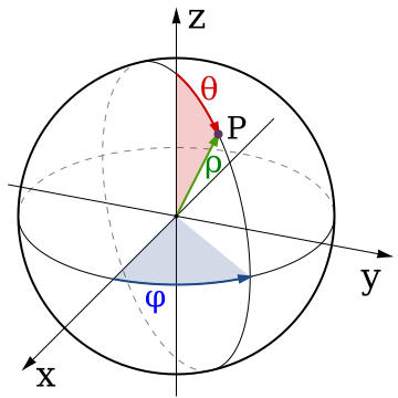
Input: angular source position in the telescope field of view
(θ, φ) measured from the optical axis
Output Coordinates: the Detector Mosaic Frame (R_MOS)
R_MOS: detector mosaic frame
(cent_y, cent_z) [mm]
2. The Datasets
The calibration data was collected for 7 optical configurations, combining grism choice and grism wheel angle (GWA).
blue grism BGS000 at 0° —
bgs000red grism RGS000 at 0° —
rgs000red grism RGS180 at 180° —
rgs180 _0 GWA tilted −4° —
_m4 GWA tilted +4° —
_p4
1st order: — many emission lines at known λ → files
*_first.csv0th order: — two compact blobs at the bandpass edges → files
*_zeroth.csv
1st-Order Spectra (Fabry-Pérot)
For each source position, we identify each line and record its PSF centroid.
39 lines from 901 nm to 1353 nm
33 lines from 1211 nm to 1866 nm
| File | Grism | GWA | Rows |
|---|---|---|---|
bgs000_0_first.csv | BGS 0° | nominal | 16 467 |
rgs000_0_first.csv | RGS 0° | nominal | 16 501 |
rgs000_m4_first.csv | RGS 0° | −4° | 14 574 |
rgs000_p4_first.csv | RGS 0° | +4° | 13 920 |
rgs180_0_first.csv | RGS 180° | nominal | 19 127 |
rgs180_m4_first.csv | RGS 180° | −4° | 13 988 |
rgs180_p4_first.csv | RGS 180° | +4° | 14 082 |
0th-Order Spectra (Two-Blob Model)
rank = 1→ assigned wavelength 1250 nm (blue edge)rank = 2→ assigned wavelength 1850 nm (red edge)
| File | Grism | GWA | Rows |
|---|---|---|---|
bgs000_0_zeroth.csv | BGS 0° | nominal | 1 426 |
rgs000_0_zeroth.csv | RGS 0° | nominal | 1 654 |
rgs000_m4_zeroth.csv | RGS 0° | −4° | 1 438 |
rgs000_p4_zeroth.csv | RGS 0° | +4° | 1 398 |
rgs180_0_zeroth.csv | RGS 180° | nominal | 1 914 |
rgs180_m4_zeroth.csv | RGS 180° | −4° | 1 394 |
rgs180_p4_zeroth.csv | RGS 180° | +4° | 1 392 |
3. Data Format — 1st-Order Files (*_first.csv)
Each row is one identified emission line from one source observation.
| Column | Frame | Unit | Description |
|---|---|---|---|
psf_id | — | — | Unique PSF identifier (traceability) |
spectra_id | — | — | Groups all lines of the same source observation |
y_nisp | NISP focal plane | mm | Source y-position from ATS encoder |
z_nisp | NISP focal plane | mm | Source z-position from ATS encoder |
| theta | Simulator frame | degrees | Azimuthal spherical angle: arctan(y_nisp / f) |
| phi | Simulator frame | degrees | Elevation spherical angle: arctan(z_nisp / f) |
| wavelength | — | nm | Fabry-Pérot etalon line wavelength (vacuum) |
| cent_y | R_MOS | mm | PSF centroid y on the detector mosaic |
| cent_z | R_MOS | mm | PSF centroid z on the detector mosaic |
| sig_y | R_MOS | mm | Centroid uncertainty along y |
| sig_z | R_MOS | mm | Centroid uncertainty along z |
Data Format — 0th-Order Files (*_zeroth.csv)
Each row is one blob (rank 1 or 2) from one source observation.
| Column | Frame | Unit | Description |
|---|---|---|---|
psf_id | — | — | Unique PSF identifier |
spectra_id | — | — | Groups both blobs of the same source |
rank | — | — | 1 = blue edge blob, 2 = red edge blob |
| wavelength | — | nm | Assigned: 1250 nm (rank 1) or 1850 nm (rank 2) |
y_nisp | NISP focal plane | mm | Source y-position from ATS encoder |
z_nisp | NISP focal plane | mm | Source z-position from ATS encoder |
| theta | Simulator frame | degrees | Azimuthal spherical angle |
| phi | Simulator frame | degrees | Elevation spherical angle |
| cent_y | R_MOS | mm | Blob centroid y on the detector mosaic |
| cent_z | R_MOS | mm | Blob centroid z on the detector mosaic |
| sig_y | R_MOS | mm | Centroid uncertainty along y |
| sig_z | R_MOS | mm | Centroid uncertainty along z |
A Quick Word on pandas
A
DataFrame is a table: rows are observations, columns are variables.It reads CSV files in one line and makes filtering, grouping, and plotting straightforward.
pd.read_csv(path)— load a CSV filedf["col"]— access a columndf[mask]— filter rows by a boolean conditiondf.groupby(...).median()— aggregatedf.describe()— summary statistics
pip install pandasDocumentation
pandas.pydata.org/docs
10-minute intro
10 minutes to pandas
Reading the Data
import pandas as pd

df = pd.read_csv("data/rgs000_0_first.csv")
print(df.shape)     # (16501, 11)
print(df.columns.tolist())
# ['psf_id', 'spectra_id', 'y_nisp', 'z_nisp', 'wavelength',
#  'cent_y', 'cent_z', 'sig_y', 'sig_z', 'theta', 'phi']
print(df.head())print(df.describe())
# Number of unique source positions
positions = df[["theta", "phi"]].drop_duplicates()
print(f"{len(positions)} unique positions")
# Wavelength range
print(f"lambda: {df['wavelength'].min():.0f} - {df['wavelength'].max():.0f} nm")spectra_id.
Working with the datasets
# All emission lines from one source observation
spectrum = df[df["spectra_id"] == df["spectra_id"].iloc[0]]
print(spectrum[["wavelength", "cent_y", "cent_z"]])sig_max = 0.05 # mm
clean = df[(df["sig_y"] < sig_max) & (df["sig_z"] < sig_max)]
print(f"{len(clean)} / {len(df)} rows kept")dz = pd.read_csv("data/rgs000_0_zeroth.csv")
print(dz.columns.tolist())
# ['psf_id','spectra_id','rank','wavelength','y_nisp','z_nisp',
# 'theta','phi','cent_y','cent_z','sig_y','sig_z']
# The two blobs of each source
blob1 = dz[dz["rank"] == 1] # blue edge (1250 nm)
blob2 = dz[dz["rank"] == 2] # red edge (1850 nm)4. Exercise — Load and Explore
Write a function that loads one 1st-order dataset, filters outliers, and returns a clean DataFrame.
import pandas as pd
import numpy as np

def load_spectra(filepath: str, sig_max: float = 0.05) -> pd.DataFrame:
    """Load and clean a 1st-order spectra dataset.

    Parameters
    ----------
    filepath : str
        Path to a *_first.csv file (e.g. 'data/rgs000_0_first.csv').
    sig_max : float
        Maximum allowed centroid uncertainty (mm).
        Rows with sig_y or sig_z above this are removed.

    Returns
    -------
    pd.DataFrame
        Cleaned DataFrame with columns:
        spectra_id, theta, phi, wavelength, cent_y, cent_z, sig_y, sig_z.

    Hints
    -----
    - Use pd.read_csv to load the file.
    - Build a boolean mask: (sig_y < sig_max) & (sig_z < sig_max).
    - Return df[mask].reset_index(drop=True).
    """
    # TODO: implement this function
    ...
Exercise (continued) — Median per Spectrum
Compute the median centroid per (spectra_id, wavelength) to reduce noise from repeated exposures.
def median_per_spectrum(df: pd.DataFrame) -> pd.DataFrame:
    """Compute the median PSF centroid per (spectra_id, wavelength).

    Parameters
    ----------
    df : pd.DataFrame
        Cleaned DataFrame returned by load_spectra().

    Returns
    -------
    pd.DataFrame
        One row per (spectra_id, wavelength), with columns:
        spectra_id, theta, phi, wavelength, cent_y, cent_z.

    Hints
    -----
    - Use df.groupby(["spectra_id", "wavelength"]).median().
    - Reset the index after groupby.
    - theta and phi are the same for all rows with the same spectra_id.
    """
    # TODO: implement this function
...Exercise (continued) — 0th-Order Centers
Load a 0th-order dataset and compute the 0th-order center for each source.
def zeroth_order_centers(filepath: str) -> pd.DataFrame:
    """Compute the 0th-order center from the two-blob model.

    Parameters
    ----------
    filepath : str
        Path to a *_zeroth.csv file.

    Returns
    -------
    pd.DataFrame
        One row per source with columns:
        spectra_id, theta, phi, cent_y, cent_z
        where cent_y and cent_z are the mean of the two blob centroids.

    Hints
    -----
    - Load with pd.read_csv.
    - Group by spectra_id and compute mean of cent_y, cent_z.
    - The mean over rank 1 and rank 2 gives the 0th-order center.
    - theta and phi are the same for both ranks: keep with .first().
    """
    # TODO: implement this function
    ...
5. Data Visualization
Visualization reveals structure, outliers, and the expected behavior.
Key questions to answer visually:
- Where are the sources in the field of view (θ, φ) in the telescope simulator frame?
- Where do their PSFs land in R_MOS (cent_y, cent_z)?
- Is the mapping smooth and regular?
- How does the GWA angle shift the spectra on the detector?
- What do the 1st-order and 0th-order positions look like relative to each other?
colored by wavelength — showing spectra as colored lines across the detector.
Exercise 1 — Plot Source Positions
Plot the unique source positions in the telescope simulator frame.
import matplotlib.pyplot as plt

def plot_field(df: pd.DataFrame, title: str = "") -> None:
    """Plot unique source positions in the simulator frame.

    Parameters
    ----------
    df : pd.DataFrame
        DataFrame with theta and phi columns.
    title : str
        Plot title.

    Hints
    -----
    - Extract unique positions: df[["theta","phi"]].drop_duplicates()
    - Use plt.scatter(pos["theta"], pos["phi"], s=10).
    - Label the axes: "theta [degrees]", "phi [degrees]".
    - Add plt.grid(True) and plt.title(title).
    - What is the angular range of the field of view?
    """
    # TODO: implement this function
...Exercise 2 — Map to Detector
Plot the PSF centroids in R_MOS, colored by wavelength or source angle.
def plot_centroids(df: pd.DataFrame, color_by: str = "wavelength") -> None:
    """Plot PSF centroid positions in R_MOS.

    Parameters
    ----------
    df : pd.DataFrame
        DataFrame with cent_y, cent_z columns.
    color_by : str
        Column name for color coding.
        Try: "wavelength", "theta", "phi".

    Hints
    -----
    - plt.scatter(df["cent_y"], df["cent_z"],
                  c=df[color_by], cmap="rainbow", s=4, theta=0.5)
    - Add plt.colorbar(label=color_by).
    - Label the axes: "cent_y [mm]", "cent_z [mm]".
    - When colored by wavelength, each source traces a line = its spectrum.
    """
    # TODO: implement this function
...Exercise 3 — Compare GWA Configurations
Overlay multiple configurations to see the effect of GWA angle on spectrum positions.
def compare_gwa(configs: list[str], labels: list[str]) -> None:
    """Overlay centroid maps from different GWA angle configurations.

    Parameters
    ----------
    configs : list[str]
        List of *_first.csv paths.
        e.g. ['data/rgs000_0_first.csv',
               'data/rgs000_m4_first.csv',
               'data/rgs000_p4_first.csv']
    labels : list[str]
        Legend labels for each dataset.

    Hints
    -----
    - For each file: load_spectra -> median_per_spectrum.
    - Plot cent_y vs cent_z for each on the same axes.
    - Use distinct colors and add plt.legend().
    - The GWA angle shifts all spectra along the dispersion direction.
    - What is the shift in mm between _0, _m4 and _p4?
    """
    # TODO: implement this function
    ...
Exercise 4 — 1st Order vs 0th Order
Overlay 1st-order spectra and 0th-order blob positions for the same configuration.
def compare_orders(config: str) -> None:
    """Compare 1st-order and 0th-order positions on the detector.

    Parameters
    ----------
    config : str
        Configuration name, e.g. 'rgs000_0'.

    Hints
    -----
    - Load data/<config>_first.csv  -> 1st-order centroids.
    - Load data/<config>_zeroth.csv -> 0th-order blob positions.
    - Plot both on the same axes with distinct colors/markers.
    - The 0th-order blobs should appear as two compact clusters,
      offset from the dispersed 1st-order spectra (~800 px away).
    - Use plt.legend(['1st order', '0th blob (rank1)', '0th blob (rank2)']).
    """
    # TODO: implement this function
...Final Goal — Spectra in R_MOS
Plot 1st-order PSF centroids in R_MOS colored by wavelength.
cent_y vs cent_z colored by wavelength. Each row of dots = one source spectrum (Fabry-Pérot lines).
def plot_spectra(df: pd.DataFrame) -> None:
    """Plot 1st-order PSF centroids in R_MOS colored by wavelength.

    Hints
    -----
    - plt.scatter(df["cent_y"], df["cent_z"],
                  c=df["wavelength"], cmap="rainbow", s=6, theta=0.5)
    - Add colorbar labeled "wavelength [nm]".
    - Try coloring by "theta" or "phi" to see the field structure.
    """
    # TODO: implement this function
    ...
Summary
| Concept | Key point |
|---|---|
| Ground test setup | NISP only — telescope simulator provides angular source positions |
| Optical chain | Telescope Simulator → Collimator → Grism → Camera → Detector |
| Input frame | Telescope simulator spherical angles (θ, φ) [degrees] |
| Output frame (R_MOS) | Detector mosaic centroids (cent_y, cent_z) [mm] |
| 1st-order datasets | 7 files *_first.csv — Fabry-Pérot lines, ~14–19k rows each |
| 0th-order datasets | 7 files *_zeroth.csv — 2 blobs per source (rank 1 & 2), ~1400–1900 rows each |
| Configurations | bgs000_0, rgs000_{0,m4,p4}, rgs180_{0,m4,p4} |
| Model target | (θ, φ, λ) → (cent_y, cent_z) |
| Quality filter | Remove rows with sig_y or sig_z above threshold (~0.05 mm) |
| Next step | Implement and calibrate the physical dispersion model (section 3) |