General Introduction
Cosmology & Spectroscopy
ANR DISPERS – Bachelor Project
Centre de Physique des Particules de Marseille (CPPM)
1. General Cosmology
From observation to the Standard Model
What is Cosmology?
Cosmology is the scientific study of the origin, evolution, and large-scale structure of the Universe as a whole.
· How did the Universe begin?
· How did it evolve over 13.8 billion years?
· What is its large-scale structure?
· What is its ultimate fate?
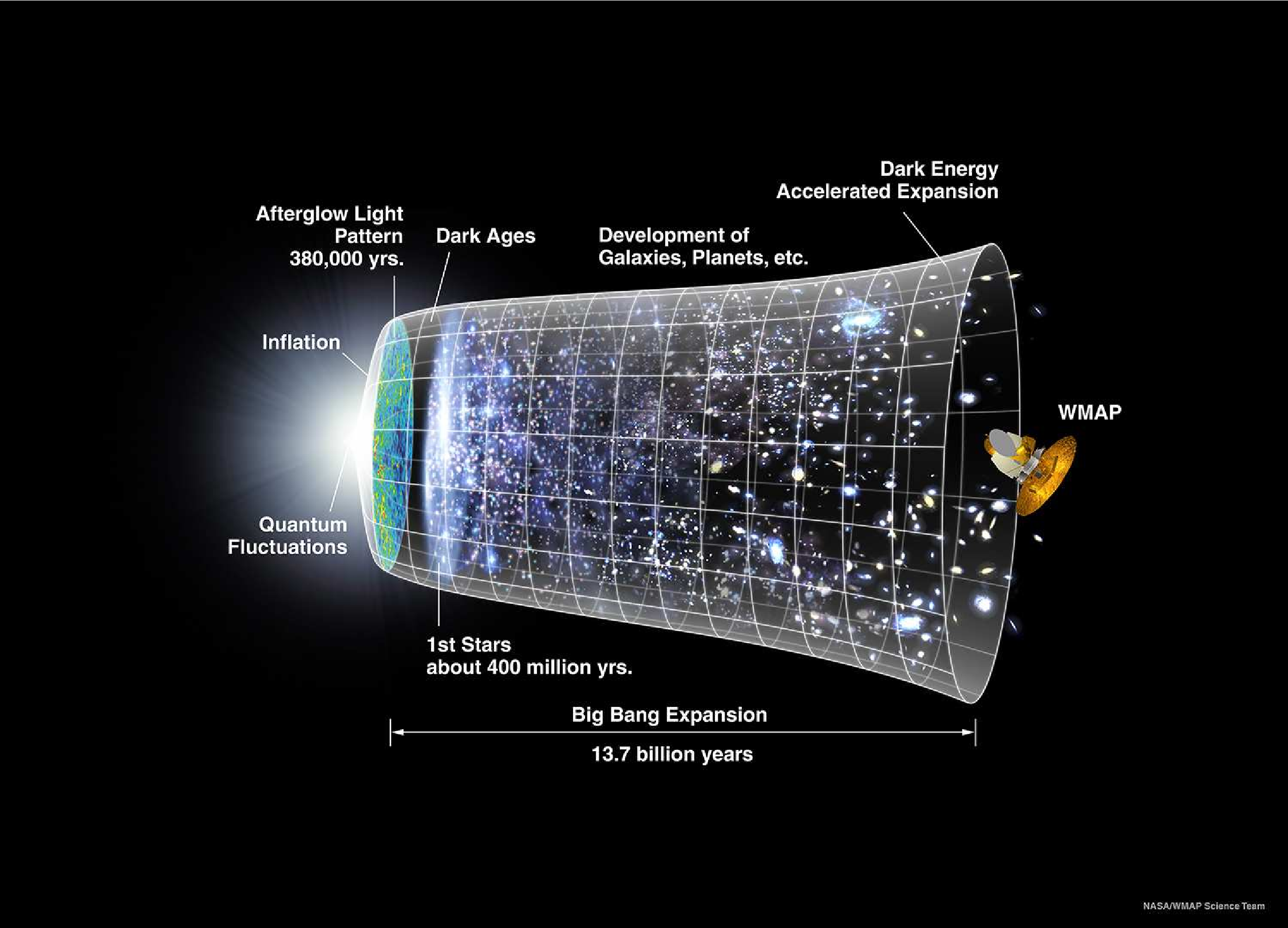
Timeline of the Universe: from the Big Bang (~10⁻³² s) through inflation, nucleosynthesis, recombination (CMB emission at z~1100), to the formation of the first stars and galaxies.
Source: NASA / WMAP Science Team
Why Use a Telescope?
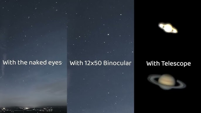
Pupil diameter: ~7 mm
Integration time: ~1/15 s
Can see ~5 000 stars with the naked eye
Mirror diameter D = 0.1 m → 10 m
Number of photons collected ∝ D²
A 1 m mirror collects ~10 000× more light than the eye!
Number of photons collected ∝ D² × t
Source: https://www.youtube.com/@science_sir
Deep Sky Imaging – Revealing the Distant Universe

JWST First Deep Field (2022). Exposure ~12 h.
Source: NASA / ESA / CSA / STScI
Each pixel records the total flux received from the sky in a broad wavelength band.
We see the shape, brightness and colour of sources.
· What the source is made of
· How fast it is moving
· How far away it is
To answer these questions, we need to disperse the light into a spectrum.
Spectroscopy – Dispersing Light

A prism disperses white light into its constituent wavelengths (colours).
A diffraction grating does the same more efficiently.
Source: Wikipedia – CC BY-SA
Each element absorbs and emits light at fixed, known wavelengths.
Hydrogen: 656 nm (H α, red), 486 nm (H β, blue-green), …
Sodium: 589 nm (yellow doublet)
Calcium, Magnesium, Oxygen, …
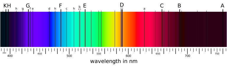
Fraunhofer absorption lines in the solar spectrum:
dark lines where atoms in the solar atmosphere absorb specific wavelengths.
Source: Wikipedia – Public domain
Redshift – The Universe is Expanding

Source: Wikipedia – Georg Wiora – CC BY-SA
Spectral lines in galaxy spectra are systematically shifted toward the red. \[ z = \frac{\lambda_\text{obs} - \lambda_\text{em}}{\lambda_\text{em}} \] The farther the galaxy, the larger the shift.
The redshift is not a Doppler effect — it is the stretching of photon wavelengths as the Universe grows.
Accelerated Expansion – Type Ia Supernovae
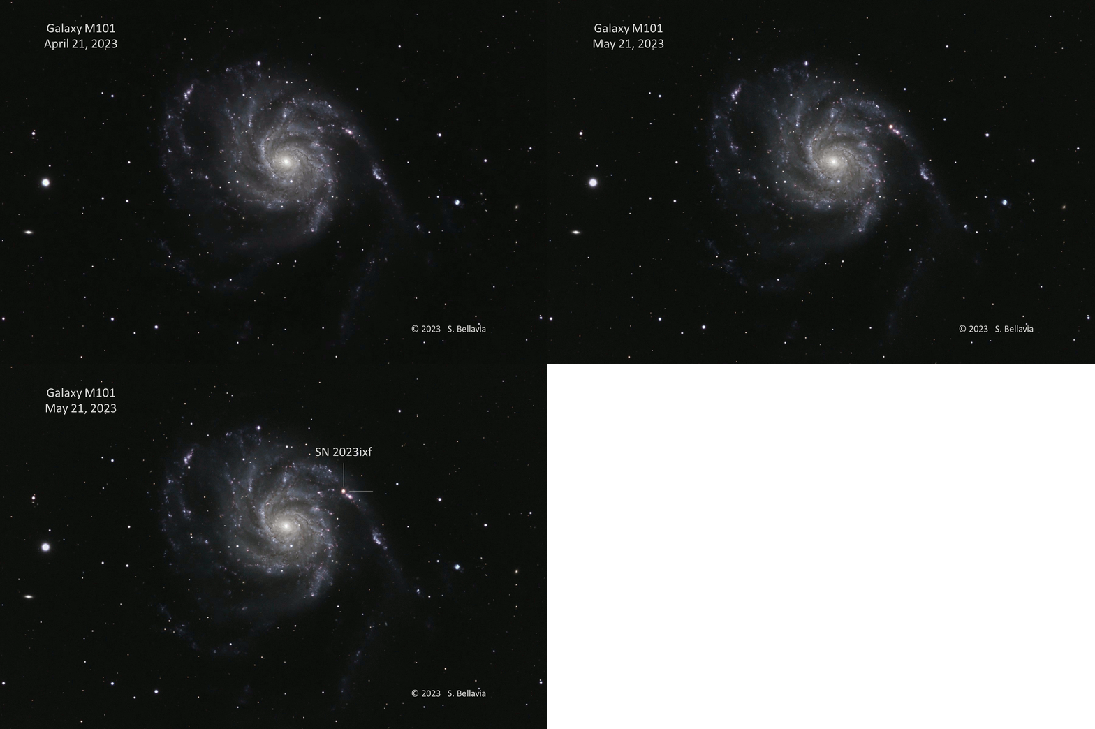
Image credit: Steven Bellavia
All Type Ia SNe have the same peak luminosity.
Measure brightness → distance.
Measure spectrum → redshift → escape velocity.
Distant SNe Ia are fainter than expected.
→ The expansion is accelerating.
Nobel Prize in Physics 2011.
The Standard Model
Homogeneity + isotropy
General Relativity
Dark energy is constant
Dark Matter is cold
+ inflation
+ initial conditions
Source: Planck Collaboration 2018, arXiv:1807.06209
The Key Questions
- Is dark energy dynamical?
- Is gravity modified on cosmological scales?
- What is the nature of dark matter? What is the neutrino mass?
- What are the initial conditions of the Universe?
2. Observational Cosmology
Probing the dark Universe with galaxies
Gravitational Lensing

LRG 3-757: a near-perfect Einstein ring produced by a massive galaxy acting as a gravitational lens (HST).
Source: NASA / ESA / HST
Mass curves spacetime.
Light follows the curved spacetime → its path is deflected near massive objects.
A very massive lens (cluster) produces multiple images, arcs, or Einstein rings.
Spectacular but rare.
A less concentrated mass distribution produces a tiny coherent distortion of background galaxy shapes.
Imperceptible on a single galaxy — but measurable statistically on millions.
Weak Lensing – Statistical Approach
Each background galaxy is distorted by ~1%.
Intrinsic galaxy ellipticity: ~30%.
A single galaxy tells us nothing — the signal is buried in noise.
Average over many galaxies in the same patch of sky:
intrinsic shapes are random and cancel out,
the coherent lensing shear adds up.

Cosmic shear field (white ticks) superimposed on the projected mass distribution from a cosmological N-body simulation.
https://arxiv.org/abs/0803.0982v1 - Figure courtesy of T. Hamana
Interactive – Gravitational Lensing Shear
nicosmo.github.io/lensing_visualization
The Cosmic Web
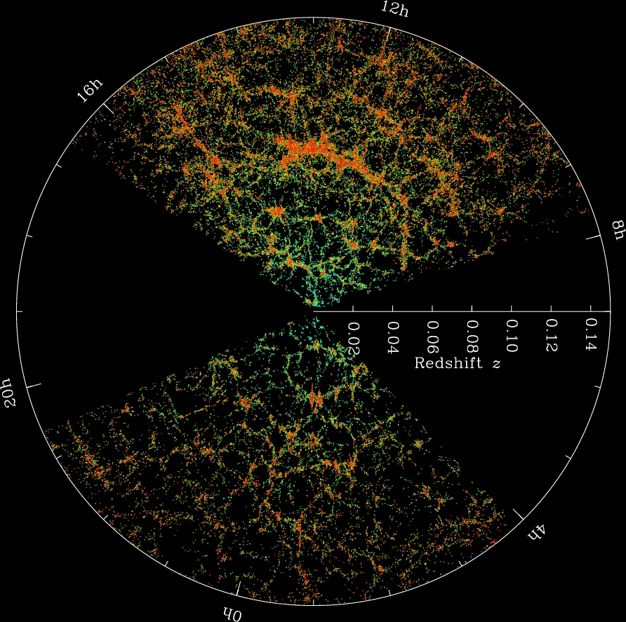
The SDSS map of the Universe. Each dot is a galaxy; the color bar shows the local density.
Credit: SDSS
They form along filaments of dark matter: the cosmic web.
The pattern encodes the initial conditions of the Universe and its subsequent evolution.
Sound waves in the early Universe left a preferred clustering scale of ~150 Mpc.
This standard ruler in the galaxy distribution measures the expansion history.
How fast structures grow depends on dark energy and gravity.
Measuring clustering at multiple redshifts tests these.
Interactive – Galaxy clustering
nicosmo.github.io/cosmic_web_explorer
Two Complementary Probes
Dark matter bends light → distorts galaxy shapes.
Map the matter distribution without seeing it.
Galaxies trace the cosmic web → galaxy positions.
Map the large-scale structure and its growth.
WL + GC measure the same underlying matter field through independent observables.
Their combination breaks degeneracies and provides the most sensitive probe of:
- Dark energy equation of state
- Growth rate of structure
- Modified gravity
- Neutrino masses
Euclid Red Book – arXiv:1610.05508
3. The Euclid Mission
Mapping the dark Universe from space
Euclid Collaboration (2022) – arXiv:1610.05508
Euclid – Why?
Improve the precision on cosmological parameters by more than one order of magnitude compared to current surveys.
Dark energy starts dominating the expansion at z ~ 0.3.
The transition epoch (z ~ 0.7–2) is where dark energy vs. dark matter competition is strongest.
This is the lever arm to constrain the dark energy equation of state w(z).
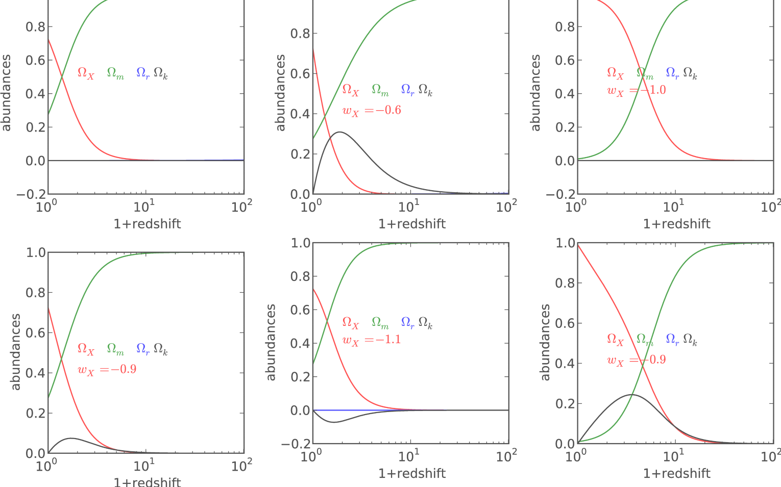
Evolution of the cosmological density parameters Ω(z) as a function of redshift, for different values of the dark energy equation of state wX. Differences between models are maximal in the range 1 < z < 2.
Source: Zoubian (2012), PhD thesis – LAM
Scientific Requirements
Coverage > 15 000 deg²
Density ≥ 30 gal/arcmin²
Redshift range: 0 < z < 2, zmed > 0.9
Shape measurement down to 0.2 arcsec
Photometric z: σ(z)/(1+z) ≤ 0.05
Coverage > 15 000 deg²
Density ≥ 3500 gal/deg²
Redshift range: 0.7 < z < 2, zmed > 1
Spectroscopic z: σ(z)/(1+z) ≤ 0.001
Purity > 80% — Completeness > 50%
Euclid Red Book – arXiv:1610.05508
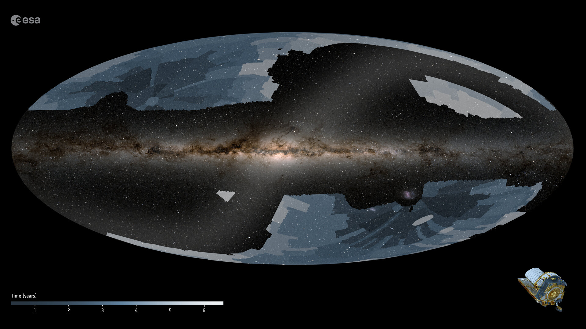
Euclid's first wide-survey field (Feb. 2024).
Each pointing ~0.55 deg² — tiled over 15 000 deg² over 6 years.
Credit: ESA / Euclid / Euclid Consortium / NASA
Why Observe from Space?
The most luminous emission line in star-forming galaxies.
Used to measure spectroscopic redshifts for GC.
\[ \lambda_\text{obs} = (1+z)\,\lambda_{H\alpha} \] At z = 0.7: λ = 1.1 μm (near-IR)
At z = 2.0: λ = 1.97 μm (near-IR)
The full target range 0.7 < z < 2 falls in the NIR.
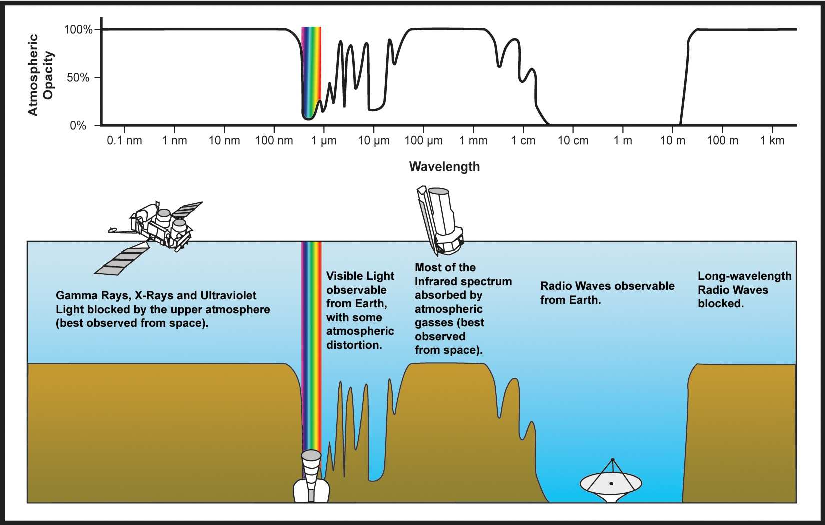
Atmospheric opacity vs. wavelength.
The NIR window (1–2 μm) is largely opaque from the ground.
A space telescope provides stable, unobstructed access.
Source: NASA
The Euclid Spacecraft
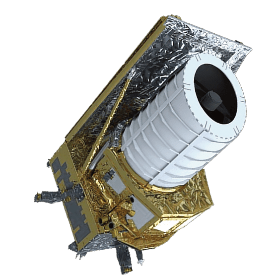
Euclid spacecraft
Launched July 1, 2023 — orbiting at the Sun–Earth L2 Lagrange point.
Credit: ESA / Euclid / Euclid Consortium / NASA / ATG medialab
Korsch three-mirror design
Primary mirror: Ø 1.2 m — f = 24.5 m
Diffraction-limited at 550 nm
1.5 million km from Earth
Stable thermal environment
No Earth/Moon occultations during survey
· VIS — Visible Imager (galaxy shapes → WL)
· NISP — Near-IR Spectrometer & Photometer (redshifts → GC)
Euclid – Payload Module
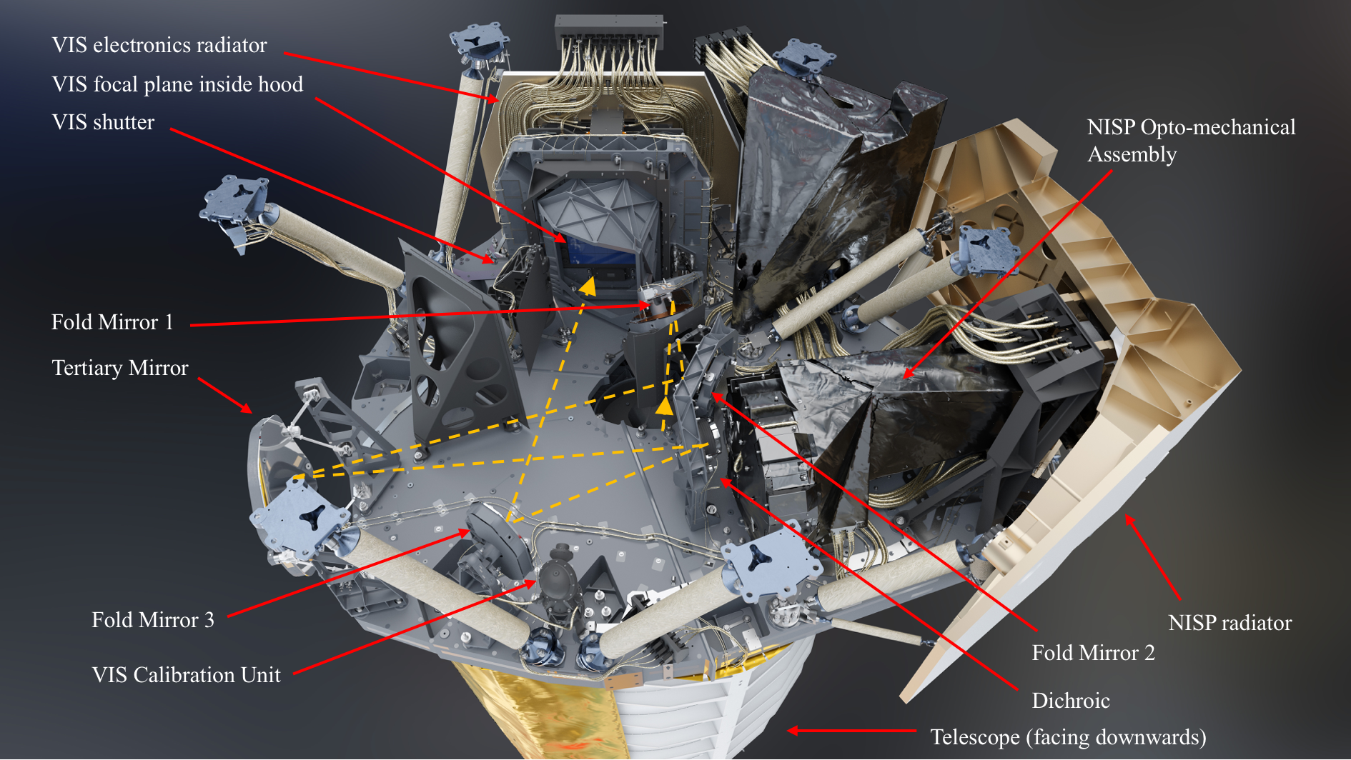
Euclid payload module: telescope + VIS + NISP on the optical bench.
Credit: Airbus / ESA / Euclid Consortium
Telescope and both instruments share a single rigid structure.
Silicon carbide (SiC) — thermally stable, low coefficient of expansion.
Temperature variation < 10 mK required.
Any PSF drift biases the weak lensing shape measurement.
VIS occupies one half of the focal plane (optical).
NISP occupies the other half (near-IR).
Both observe simultaneously for every pointing.
VIS – Visible Imager
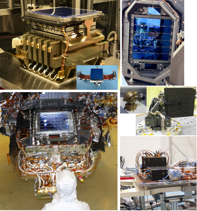
The VIS focal plane: 36 CCDs in a 6×6 mosaic — 609 Mpix total.
Credit: M. Cropper / UCL / Euclid Consortium
Measure the shape of ~1.5 billion galaxies
to reconstruct the dark matter distribution via cosmic shear.
FoV: 0.787 × 0.709 deg²
Broad optical band IE: 550–900 nm
Pixel scale: 0.1 arcsec/pixel
Depth: IE = 24.5 (SNR = 10)
PSF FWHM ≈ 0.2 arcsec
PSF must be known to <0.1% to avoid shape bias.
Any optical distortion or detector effect — charge diffusion, CTI — must be modeled.
NISP – Near-IR Spectrometer & Photometer
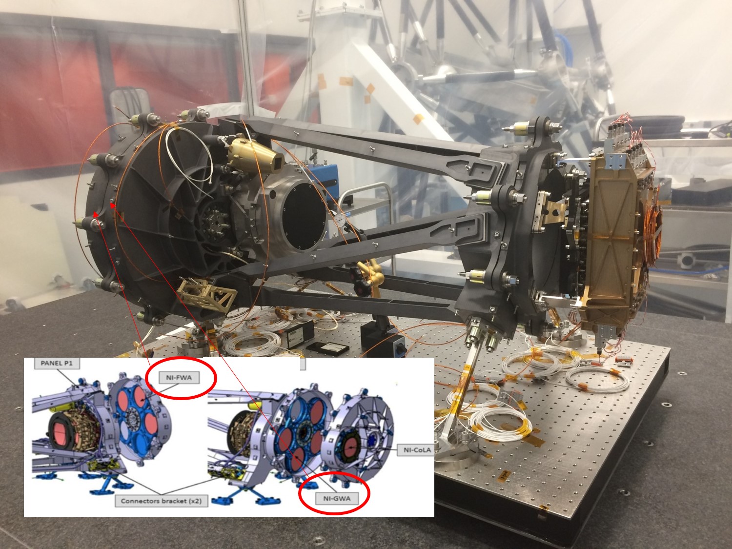
The NISP instrument during assembly at CEA/IRFU (Saclay).
Credit: CEA / IRFU
Measure spectroscopic redshifts of ~35 million galaxies via Hα (6563 Å) redshifted into the NIR: 0.9 < z < 1.8.
Filters Y, J, H — 920 to 2000 nm
16 HgCdTe arrays (2k×2k), pixel = 0.3 arcsec
Blue grism: 920–1250 nm
Red grisms: 1250–1850 nm
Spectral resolution R ≈ 380
Required: σ(z)/(1+z) ≤ 0.001
The grism wavelength calibration is the focus of this project.
4. NISP in Practice
What the detector actually sees
NISP grism image
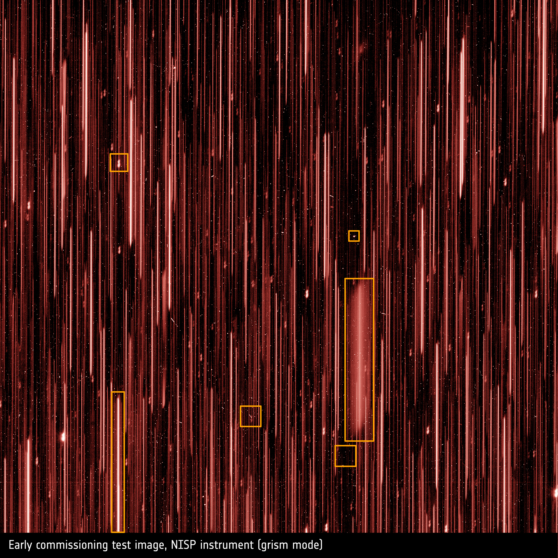
Credit: ESA / Euclid / Euclid Consortium / NASA
1st-order dispersed light – Star

Credit: ESA / Euclid / Euclid Consortium
1st-order dispersed light – Galaxy

Credit: ESA / Euclid / Euclid Consortium
0th-order dispersed light – Star

Credit: ESA / Euclid / Euclid Consortium
Artefact – Cosmic Ray Streak

Credit: ESA / Euclid / Euclid Consortium
Artefact – Hot Pixels

Credit: ESA / Euclid / Euclid Consortium
Artefact – "Snowball"

Credit: ESA / Euclid / Euclid Consortium
5. Dispersion
From photons to wavelengths on a detector
What is Dispersion?
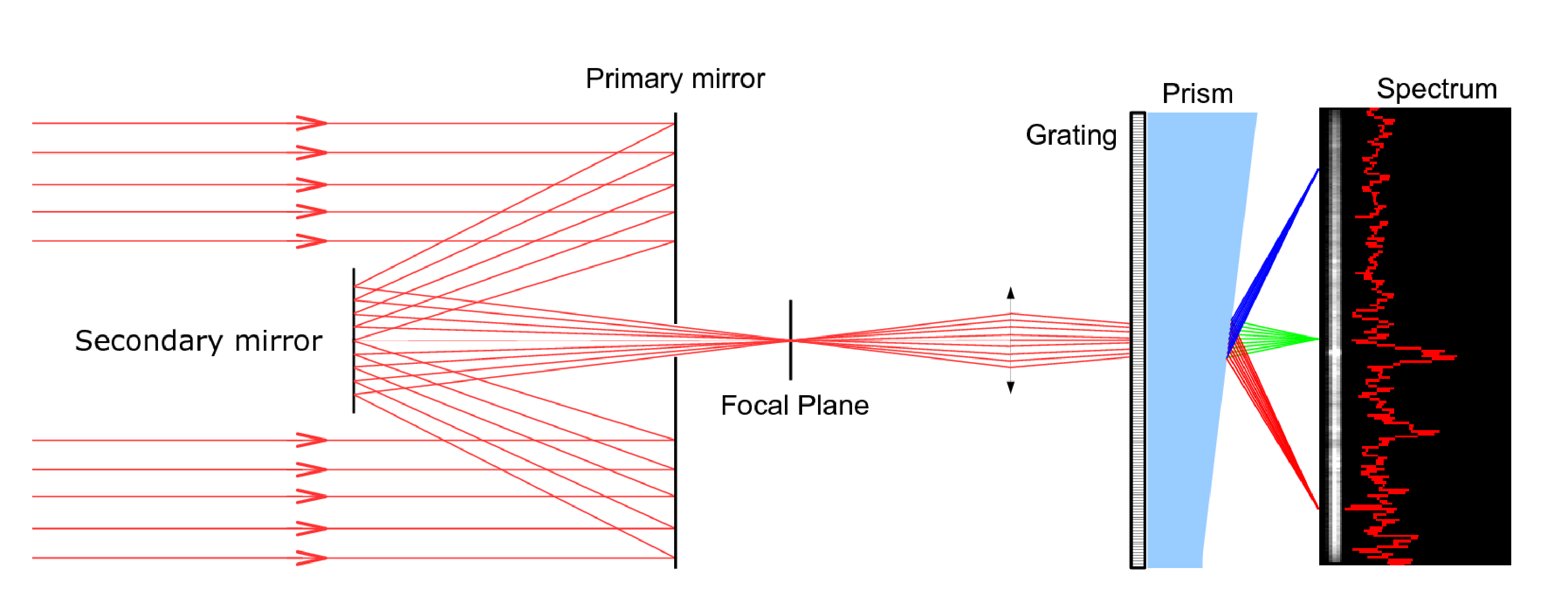
Principle of a dispersing telescope: light collected by the primary mirror, redirected by the secondary, then dispersed by a grism onto the detector. Each wavelength hits a different pixel.
A grism (grating + prism) deflects each wavelength λ by a different angle → different position on the detector.
\[ x_\text{det} = f(x_0) + D(\lambda - \lambda_0) \] The pixel position along the dispersion axis is a direct measure of wavelength.
Measuring position → redshift.
Why does accuracy matter?
Δλ/λ ~ 1/380 → Δz ~ 0.003
Required: σ(z)/(1+z) ≤ 0.001
Sub-pixel precision is mandatory.
Dispersion on the Detector
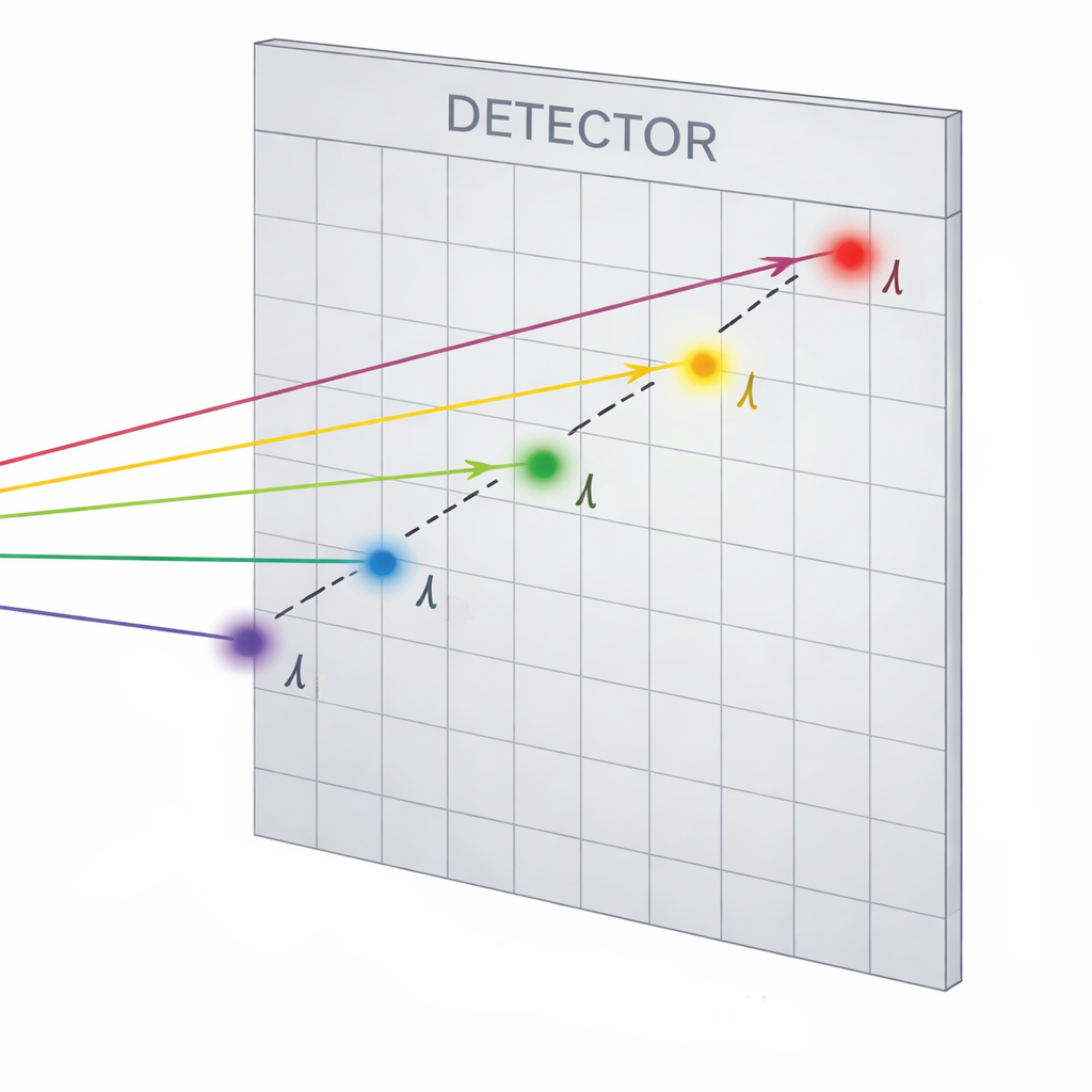
Each source produces a spectrum on the detector: its pixels are displaced along the dispersion direction by an amount that depends on wavelength λ. The position on the detector encodes the redshift.
Given a source at position (α, δ) on the sky, the photon of wavelength λ lands at detector position (x, y).
The dispersion model is the function:
\[ (x,\, y) = f\!\left(\alpha,\, \delta,\, \lambda\right) \]
· the optical design of the telescope
· the grism angle and groove density
· the position of the source in the field of view
· temperature, alignment, aberrations
Build an accurate model of f(α, δ, λ) → (x, y) across the full NISP field of view.
Slitless Spectroscopy – How It Works
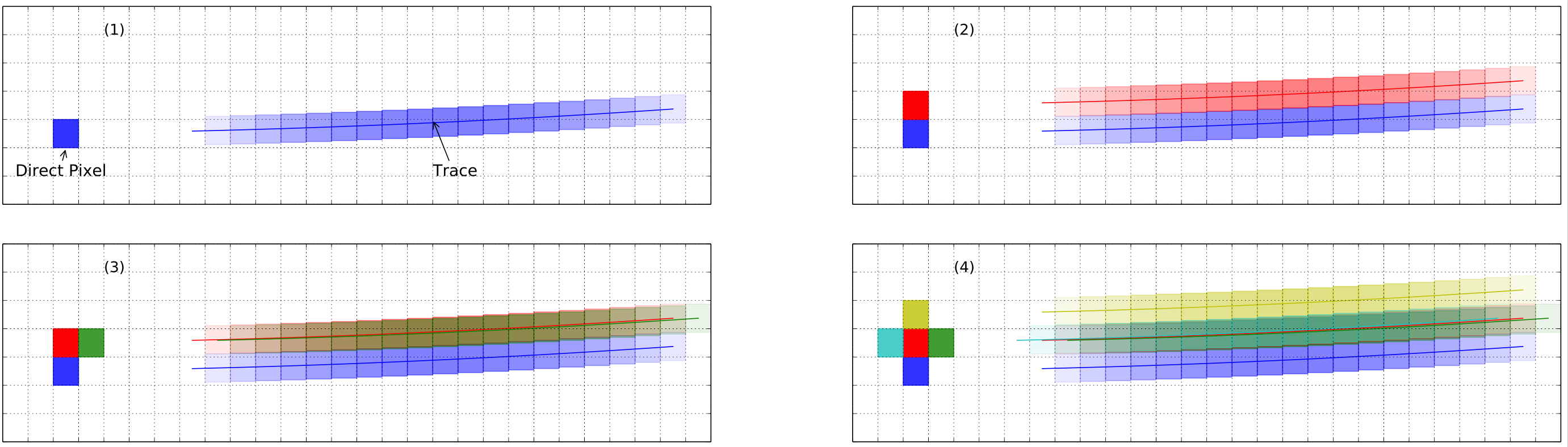
In slitless mode the disperser is placed in the full beam: every object is dispersed simultaneously. For extended sources, light from adjacent pixels overlaps in the dispersion direction, reducing the effective spectral resolution.
Credit: JWST documentation
Each pixel of a galaxy emits its own spectrum. These spectra overlap in the dispersion direction
Effective spectral resolution is reduced for large galaxies.
Slitless Spectroscopy – Contamination
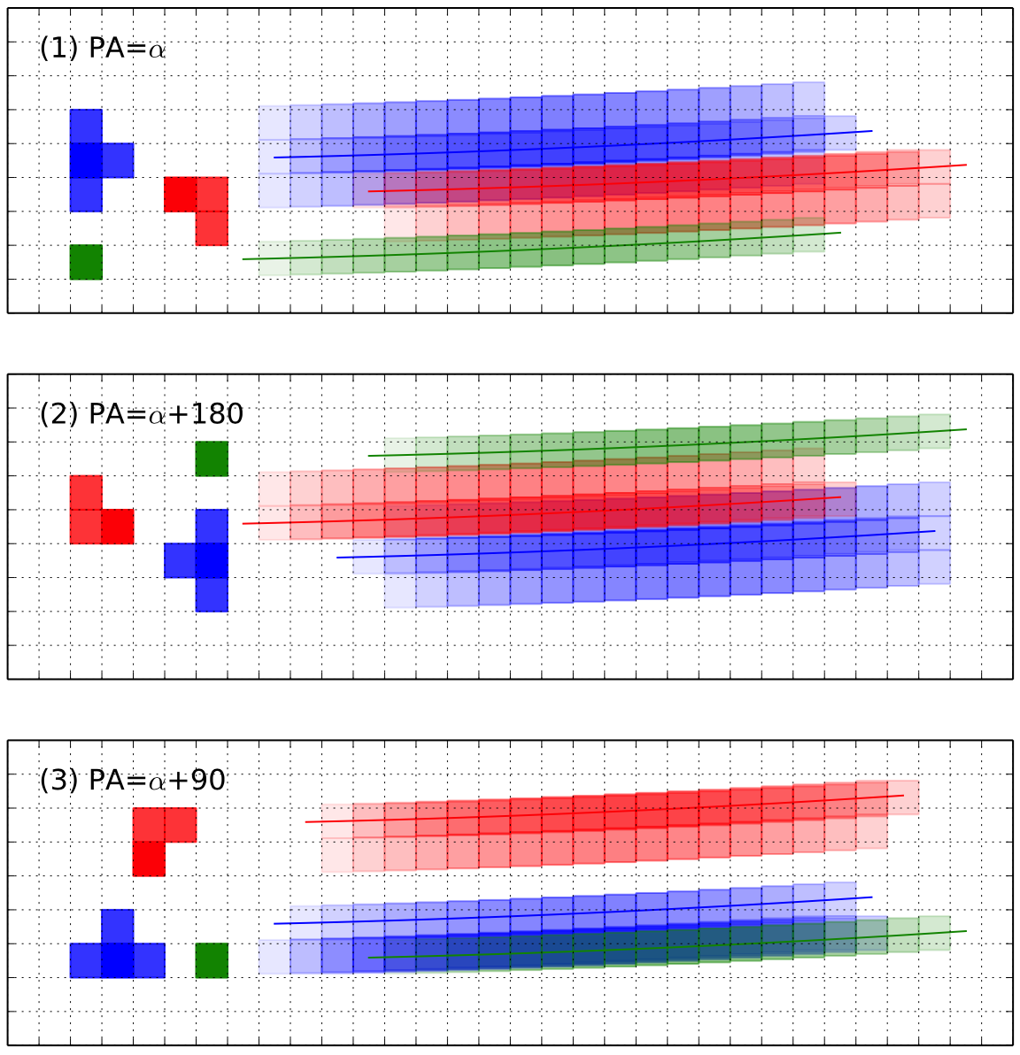
Since all objects are dispersed in the same direction, spectra of nearby sources can overlap. Observing at different sky position angles changes which spectra contaminate each other — enabling decontamination by combining multiple exposures.
Credit: JWST documentation
A neighbour projected along the dispersion direction will have its spectrum overlap with the target's.
This biases the measured flux — and therefore the redshift.
4 exposures with the grism at different orientations Contamination patterns change → can be identified and removed.
To predict where each spectrum falls on the detector, and therefore which sources contaminate which.
6. Your Project
Modelling the NISP dispersion
Roadmap
- Intro data – Explore the NISP calibration data: spectra, traces, wavelength solutions
- Intro model – Build a physical dispersion model: f(α, δ, λ) → (x, y)
- Intro ML – Learn the residuals: apply machine learning to correct the model
- Projet – Evaluate the hybrid model on real calibration data
→ predicted detector position (x, y)